A Model of an Oscillatory Neural Network with Multilevel Neurons for Pattern Recognition and Computing


Institute of Physics and Technology, Petrozavodsk State University, 31 Lenina str., 185910 Petrozavodsk, Russia
*
Author to whom correspondence should be addressed.
Electronics 2019, 8(1), 75; https://doi.org/10.3390/electronics8010075
Submission received: 20 November 2018
/
Revised: 1 January 2019
/
Accepted: 5 January 2019
/
Published: 9 January 2019
(This article belongs to the Special Issue Energy-Efficient and Reliable Information Processing: Computing and Storage)
Abstract
:The current study uses a novel method of multilevel neurons and high order synchronization effects described by a family of special metrics, for pattern recognition in an oscillatory neural network (ONN). The output oscillator (neuron) of the network has multilevel variations in its synchronization value with the reference oscillator, and allows classification of an input pattern into a set of classes. The ONN model is implemented on thermally-coupled vanadium dioxide oscillators. The ONN is trained by the simulated annealing algorithm for selection of the network parameters. The results demonstrate that ONN is capable of classifying 512 visual patterns (as a cell array 3 × 3, distributed by symmetry into 102 classes) into a set of classes with a maximum number of elements up to fourteen. The classification capability of the network depends on the interior noise level and synchronization effectiveness parameter. The model allows for designing multilevel output cascades of neural networks with high net data throughput. The presented method can be applied in ONNs with various coupling mechanisms and oscillator topology.
1. Introduction
Hypotheses about the functional importance of synchronization for information processed by the brain were put forward long ago [1,2] and its experimental discovery [3,4] encouraged the creation of neural networks models with oscillatory dynamics [5,6,7] and neuromorphic algorithms of image processing based on synchronization [8,9,10,11].
Research on ONN is mainly based on phase oscillator models. Such models, primarily the Kuramoto model [12], have been very useful for studying systems of various topology with a large number (N > 103) of oscillators, where not only global synchronization but the synchronization by middle field [13], mode of quasi-synchronization [14] and even chimeras synchronization [15] are feasible.
Recently, the problem of pattern recognition in ONN has been intensively studied [16,17], and two main global synchronization methods have been outlined: frequency-shift [10] and phase-shift [11] keying methods. Frequency encoding, based on synchronized frequency shift [10], allows usage of an oscillator star configuration and N couplings; however, the disadvantage of this method is that only it stores a single pattern. The phase-shift keying method of encoding [11] enables storage of more than one pattern by certain combinations of phase shift at the same weight ONN matrix. However, this method has the following drawbacks: N2 couplings with tunable weights and a two-stage procedure of pattern recognition.
Another class of ONN is based on relaxation oscillators that generate multiple pulses of short duration and fixed amplitude. Such pulses (spikes) can code information at pulse-repetition frequency. An important distinguishing feature of a pulse type ONN from classic spiking neural networks (SNN) is a self-oscillating mode of ONN neuro-oscillators. This mode is not indicative for SNNs and real (biological) neurons, which are characterized by a forced response through generation of a single spike or their group, when the neuron threshold level is achieved. However, ONNs are fascinating due to the simplicity of the hardware implementation as available advanced micro- and nano-electronic self-oscillators ensure the compact size and energy efficiency of the circuit.
Pulse type ONNs with a multi-frequent spectrum of periodic oscillation feature a specific mode of multiple frequency synchronization, or in other words, a high order synchronization effect [18] (harmonic locking [6]). We demonstrated this effect experimentally by using thermally-coupled vanadium dioxide (VO2) oscillators [19]. In relaxation oscillators with VO2-based film elements, electric self-oscillations are activated by the effect of electric switching governed by metal—insulator transition (MIT) [20,21,22,23]. The processing speed of VO2 devices switching which amounts to ~10 ns [24] and manufacturing technology that allows switching elements to be created with high levels of nano-scalability make VO2-switch based oscillators the perfect objects for research on neuro-oscillators to solve cognitive technology problems [25,26,27,28]. Relaxation oscillators with high order synchronization effects can be realized by using electric coupling [25,26,27,28] and by using not only VO2-switches, but any other switching elements such as thyristors [29], tunneling diodes [30], resistive memory cells [31], and spin torque oscillator [16,32].
In this paper, we studied the ONN of thermally-coupled VO2-oscillators and present a general concept of visual pattern recognition based on high order synchronization effects. We used the multiplicity of synchronous states to extract object classes by using a single output oscillator (compared to, for example, an array of oscillators at the output [10,11]). The concept of a multi-level neuron allows for using a smaller number of output neurons (oscillators) to implement the more complex cognitive functions of the neural network. We developed a set of special metrics [19,33], such as the high-order synchronization value and the synchronization effectiveness value. Compared to the neural network presented in [33], this network is able not only to memorize and classify patterns, but also to perform logical operations, computer calculations and emulate other functions of artificial intelligence systems.
2. Materials and Methods
2.1. Oscillator Circuit and Method of ONN Organization
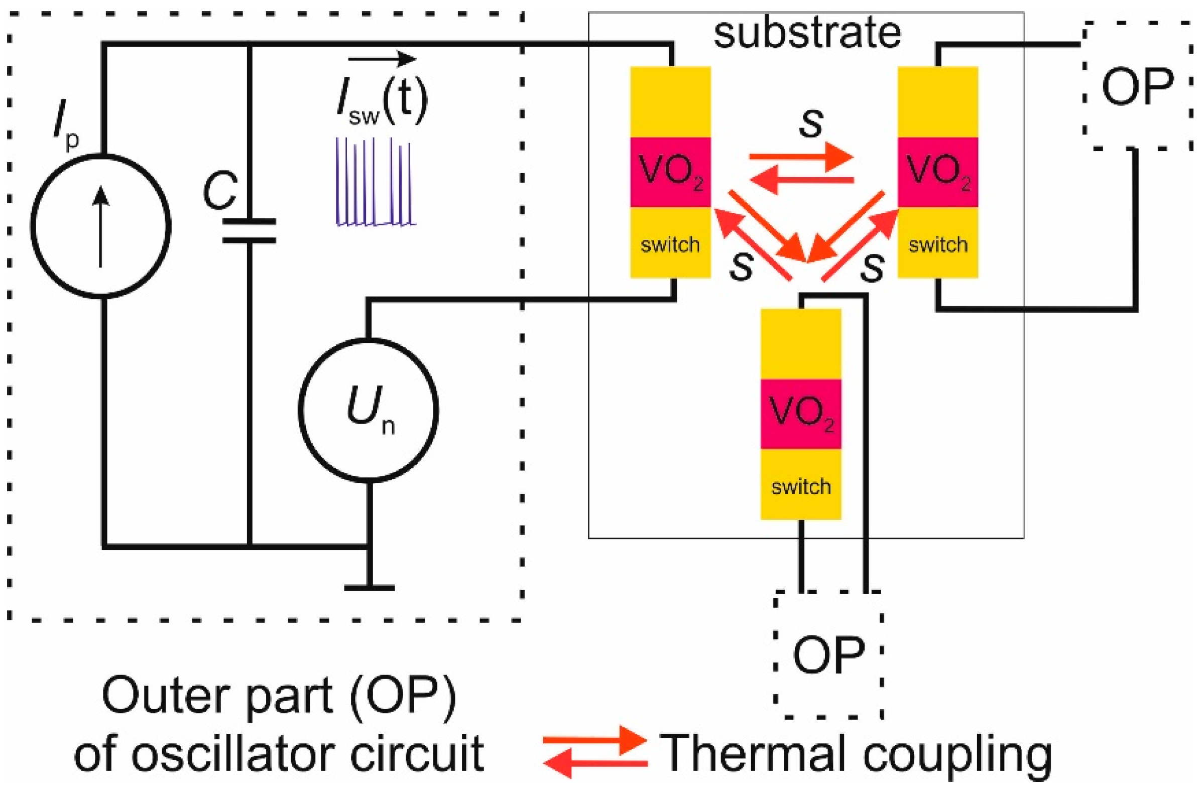
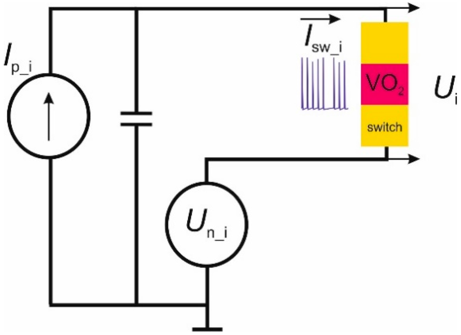
The basic element in the studied ONN is an oscillator implemented on the circuit of a relaxation generator (Figure 1) based on a VO2-switch. We described the process of fabrication and electric I–V characteristics of an electric VO2-switch in detail in [19]. I-V characteristics are well approximated by a piecewise linear function (see Appendix A.1) that has two conduction states (low-resistance and high-resistance) and a region of negative differential resistance (NDR). These switches may be used in the circuit of a relaxation generator with power supply Ip holding the operation point in the NDR region of the I-V characteristic and with capacity C, connected to the switch in parallel. In addition, a source of noise Un models the circuit’s interior or exterior noises, such as current noise of a switch [34]. The oscillator’s output signal is current Isw(t) flowing through the VO2-switch, which is used to calculate the synchronization level of two oscillators (see Section 2.3). The current signal directly determines the effect of thermal coupling inside the network.
We applied thermal coupling to connect oscillators in a network. The presence of the thermal coupling mechanism between two VO2 oscillators was convincingly demonstrated by us in the experiment [19], and it is based on the mutual thermal effect of switches due to their Joule heating and the dependence of the threshold voltage Uth on temperature. In the pre-threshold mode, when the VO2 temperature of the switch channel is close to the MIT temperature Tth ~ 340 K [23], the external thermal influence can “push” it to switch, which is equivalent to lowering the threshold voltage by the value of s, the thermal interaction force. The switching causes an even higher temperature rise in the switch, which leads to the appearance of a temperature pulse in the surrounding space, which propagates as a temperature wave. In the oscillator circuit, the thermal effect of the switches on each other occur in the mode of repetitive pulses initiated by self-oscillations of oscillator currents, which ultimately leads to their synchronization [19]. The value of s can be controlled experimentally, for example, by varying the distances between the switches or by varying the parameters of the external circuit [19].
The choice of this coupling type is determined by the simplicity of a computing model when oscillators are electrically separated from each other, unlike in capacitive or resistive couplings [21,22,25,28]. An example of an oscillators’ interaction via thermal coupling of VO2 switches is shown in Figure 1. A detailed presentation of the mathematical model of thermally coupled relaxation oscillators is given in Appendix A.1.
The heat assisted model we used completely describes the experimental data previously observed [19,35,36]. Indeed, the speed of propagation of a thermal wave can be taken into account, but this is not in the scope of the current paper because we operated at low oscillation frequencies where the time delay is insignificant. We considered the radius of thermal interaction RTC in [19], therefore, in this model we limited ourselves to interaction with the nearest oscillators. Consideration of more complex cases can be done in future publications.
We used the concept of one-way thermal coupling of oscillators in the numerical model. This can be physically implemented when a resistance heater is used as a connecting element in one of the circuits instead of a switch [19].
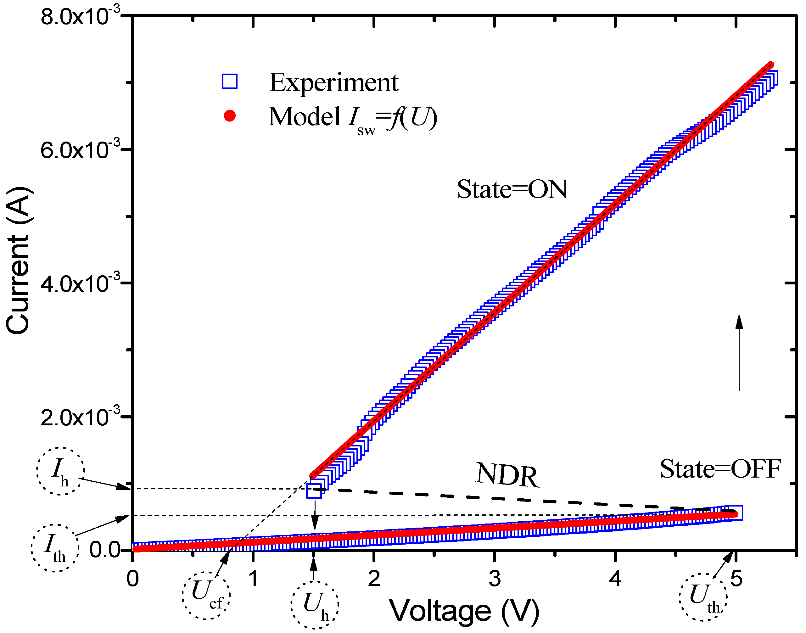
For numerical modeling we used the following parameters as I-V characteristics (Uth = 5 V, Uh = 1.5 V, Ubv = 0.82 V, Roff = 9.1 kΩ, Ron = 615 Ω). In this circuit, capacity is a constant parameter C = 100 nF, and its value significantly determines the frequency range of oscillator operation [37] and its natural frequency F0. In our case, the frequency range was 165 Hz ≤ F0 ≤ 1266 Hz at the range of feeding currents 550 µA ≤ Ip ≤ 1061 µA.
2.2. ONN Structure
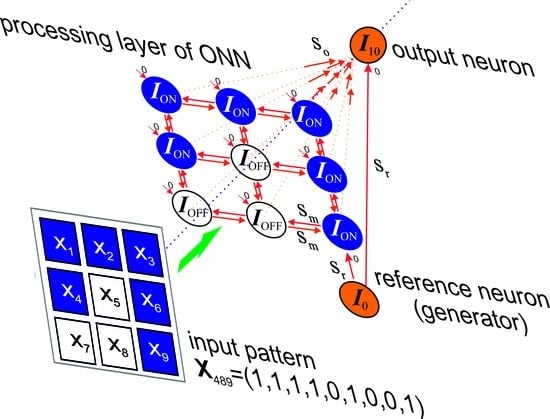
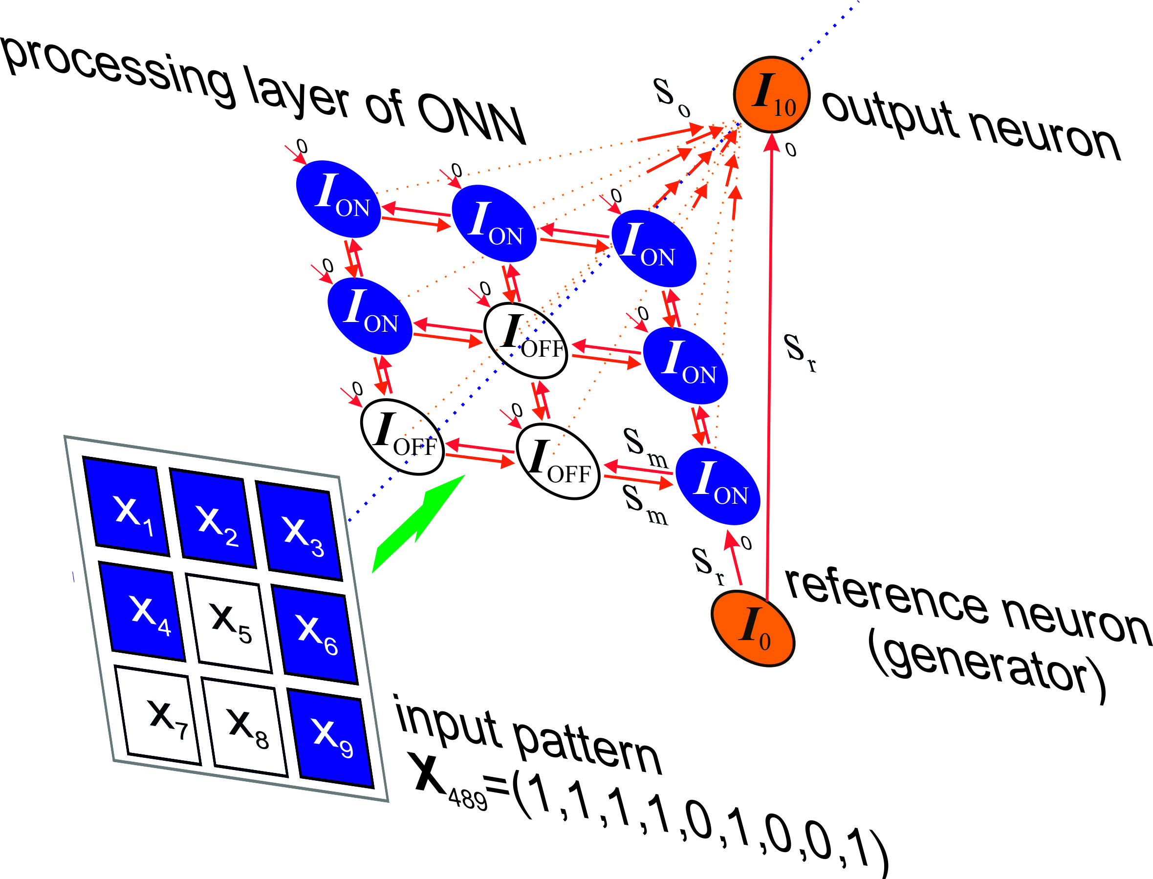
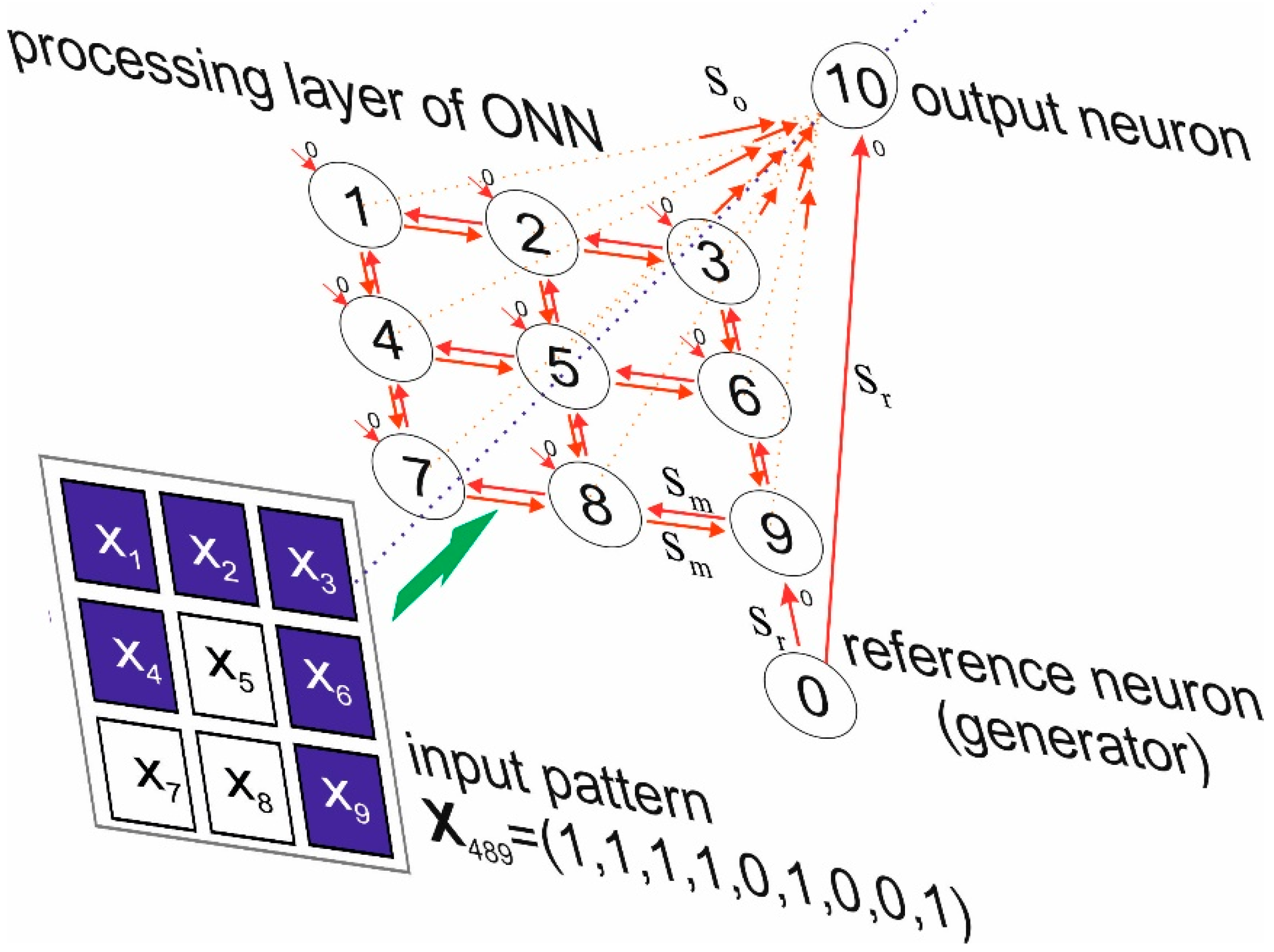
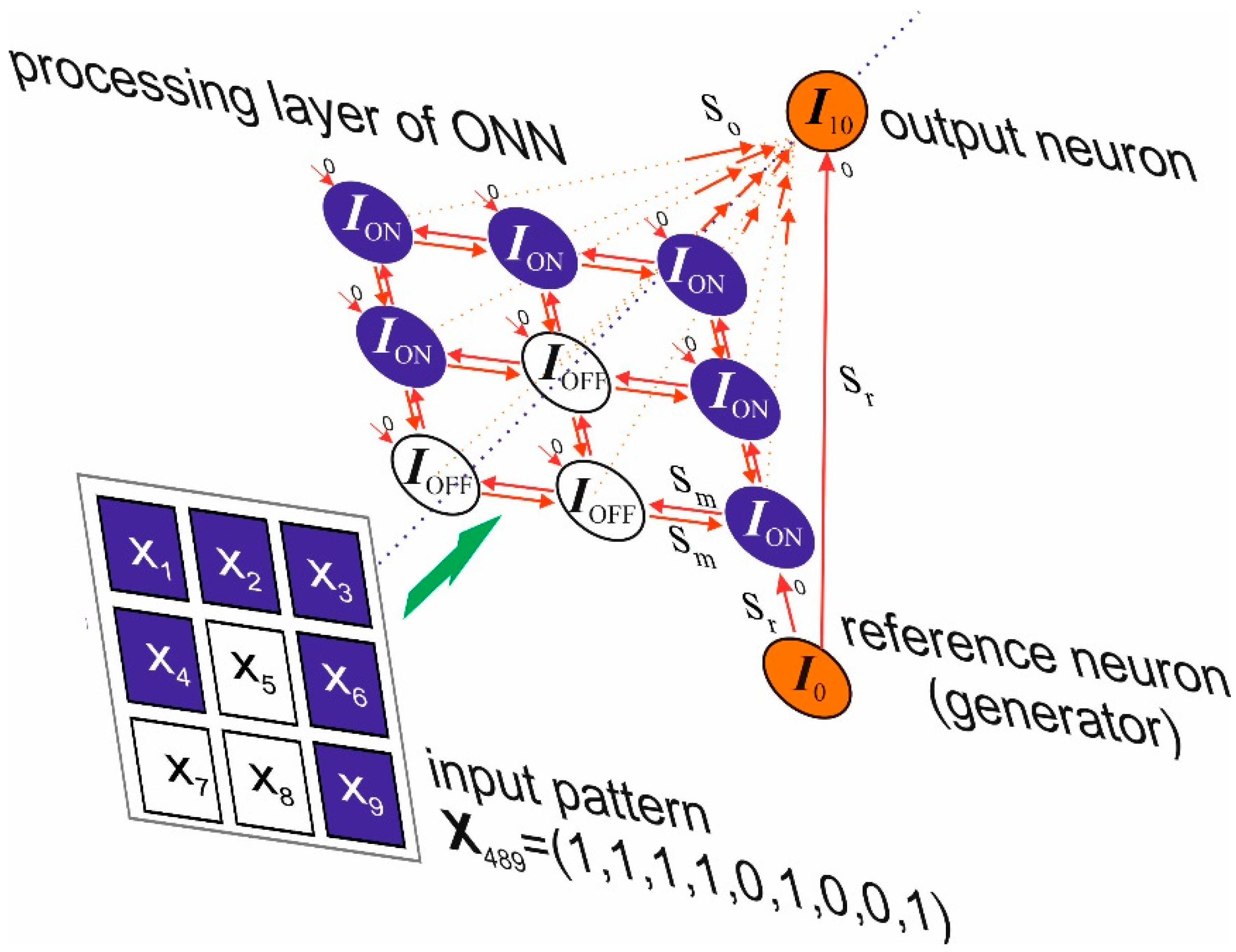
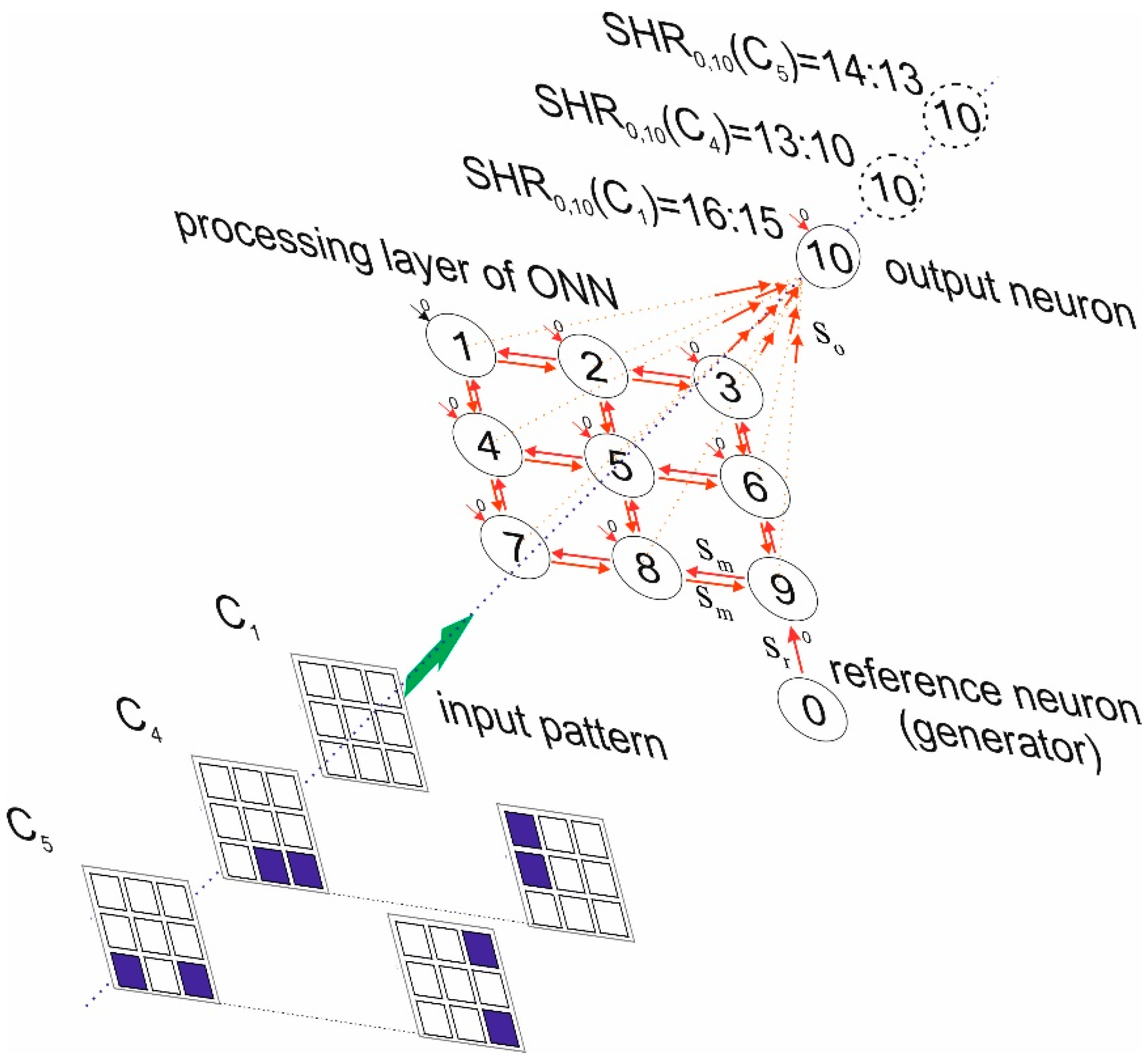
The studied ONN consists of an input pattern, which is transferred as a 3 × 3 matrix on the layer of processing neurons consisting of 9 oscillators, and of an output layer with only one oscillator (output neuron) No.10 (see Figure 2).
The magnitude of the effect of the i-th oscillator on the j-th oscillator is determined by coupling strength si,j, that is set by the following matrix:
The layer of processing neurons consists of a 3 × 3 oscillator matrix connected by similar couplings (si,j = sj,i = sm, where i, j are the numbers of neighboring oscillators). Neighboring oscillators are only connected by horizontal and vertical lines. So, the central oscillator No.5 has four couplings in the matrix, the corner oscillators have two couplings, and the oscillators in the center of the edges have three couplings (with the central oscillator and two corner ones) and they all unidirectionally affect oscillator No.10 (output neuron) in the output layer (si,10 = so and s10,i = 0, where i = 1 … 9). Importantly, there is the reference oscillator No.0 in the circuit and the synchronization order of all other oscillators is measured against this oscillator. Oscillator No.0 (Figure 2) unidirectionally affects all other oscillators (s0,i = sr, and si,0 = 0, where i = 1 … 10).
The input pattern (see Figure 3) is transferred to the processing layer by selection of the feeding currents of the oscillator matrix:
where i = 1 … 9, xi are the coordinates of the input vector X = (x1, …, x9), that correspond to white (xi = 0) and blue (xi = 1) colors of pattern squares.
Transfer of the pattern to the intermediate layer causes the change in the oscillators’ feeding currents, and in turn, it leads to the change in synchronization state for all oscillators (No.1–10). The synchronization order SHR0,10 between the reference oscillator No.0 and the oscillator in the output layer No.10 serves as the control value. The values of the feeding currents for these oscillators are fixed and may differ from currents in the matrix, therefore they are indicated as I0 and I10 (see Figure 3).
2.3. Method of Synchronization Order Definition
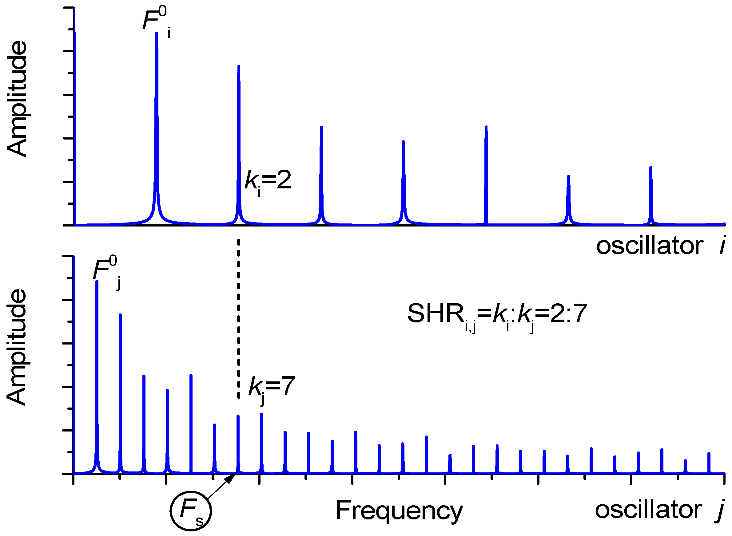
In this section, we present the method of calculating a family of metrics [19] to determine the high order synchronization of two oscillators. A family of metrics has two basic parameters: the ratio of subharmonics (SHR) and synchronization effectiveness η. In a general case, it is possible to use the concept of subharmonics ratio between oscillators i and j, which is defined [18] as a simple fraction
where ki and kj are harmonics order of oscillators at the common frequency of their synchronization Fs.
In other words, Equation (3) uses spectral approaches to describe synchronization of the higher order ki:kj, when the following relation is observed:
where Fi0, Fj0 are frequencies of main harmonics.
As an example, Figure 4 shows the qualitative spectra of two oscillators at SHRi,j = 2:7
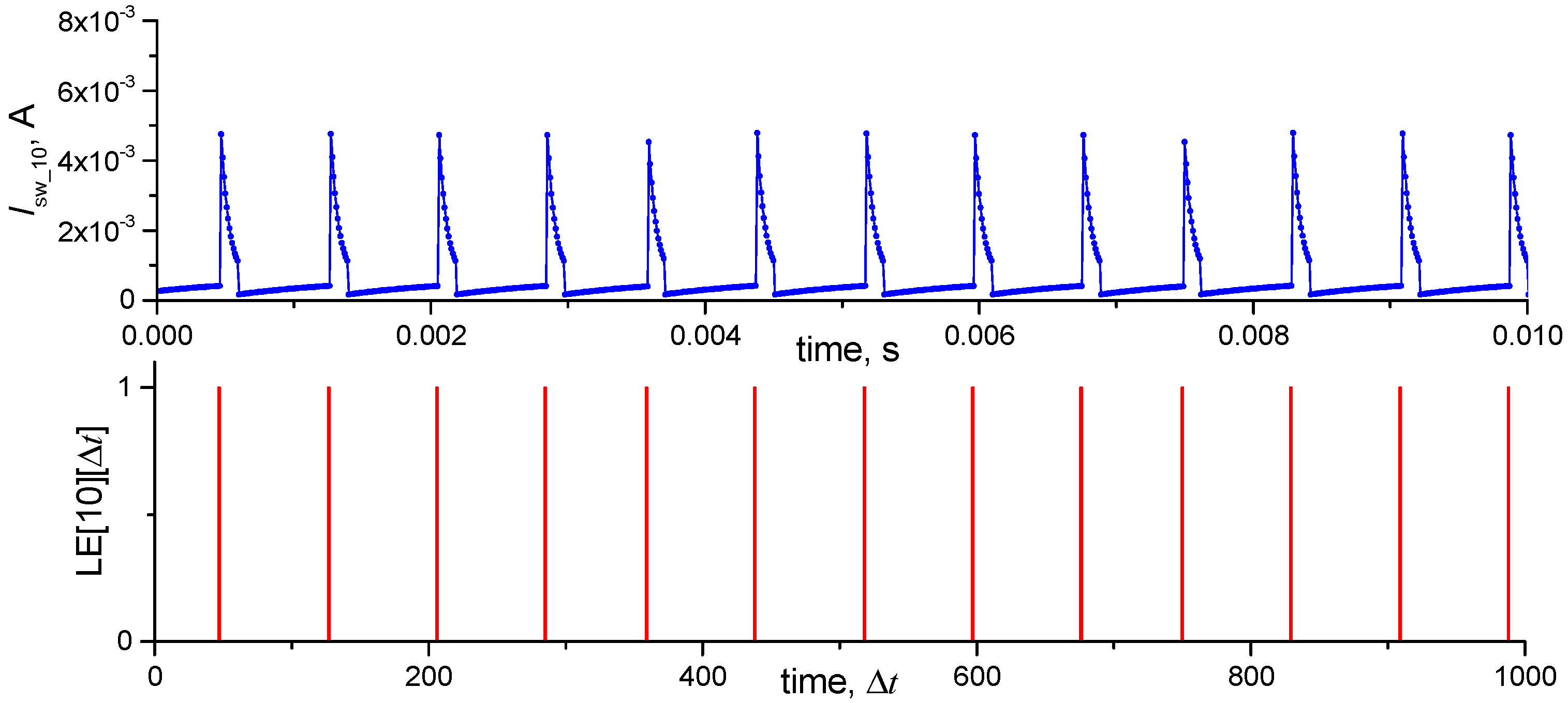
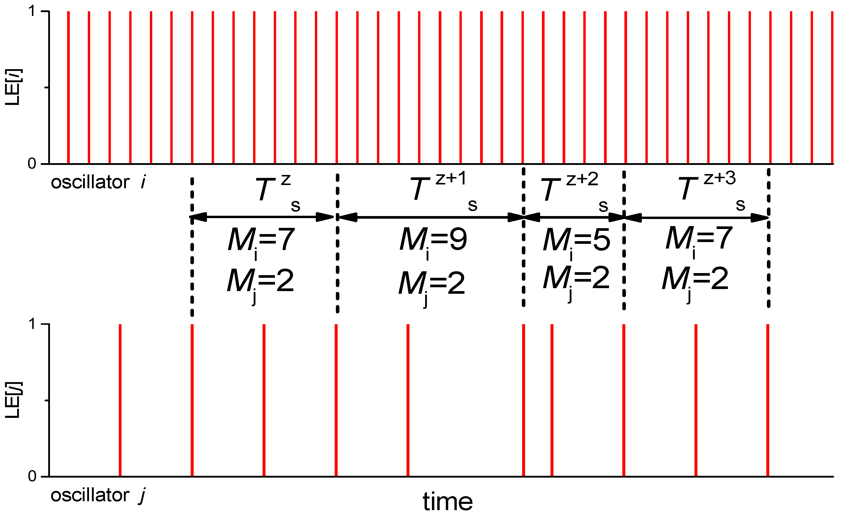
In addition, Figure 4 shows the total synchronization frequency Fs and subharmonics numbers at this frequency ki = 2 and kj = 7. Usage of signal spectra for estimating the magnitude of SHRi,j is not effective because the signals might not have a strictly periodic sequence and when noise is added to the system, the spectral lines broaden. Below, we will describe the mathematical procedure that estimates the value of SHRi,j without the use of spectral characteristics but using a current signal and array LE. Array LE stores information on the position of the current pulse leading edges (see Figure 5).
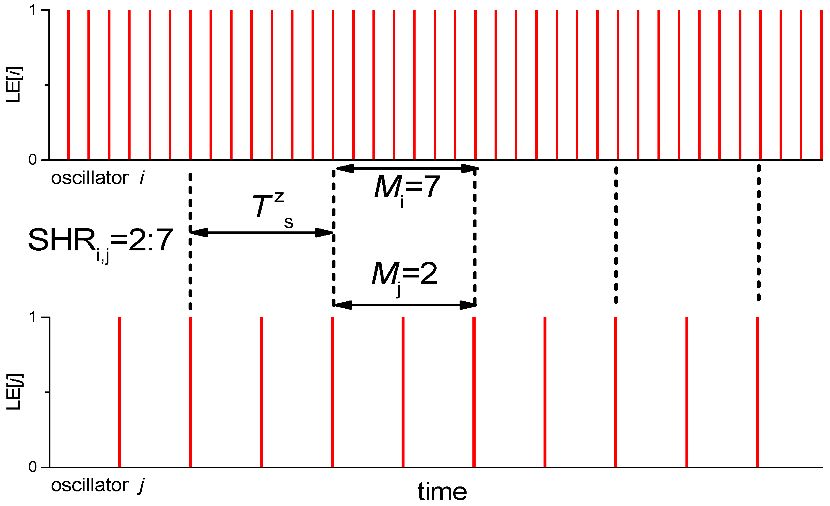
Figure 6 shows arrays LE[i] and LE[j] for two oscillators that correspond to the same ratio of the basic frequencies as shown in the spectra in Figure 4. The distance between two nearest phase-locked pulses is denoted as Tzs—the period of synchronization (where z is a conditional number of periods Ts).
Therefore, SHRi,j may be estimated using a phase-locking method:
where Mi and Mj are the number of signal periods falling into the synchronization periods Tzs of two oscillators. Formula (5) can be easily obtained from Formula (3) taking into account Formula (4) and the following ratio (Ts = Mi·Ti0 = Mj·Tj0, Fi0 = 1/Ti0, Fj0 = 1/Tj0).
In general, especially when a system behaves erratically, synchronization periods differ and spread in Tzs ≠ Tz+1s and the values of Mi and Mj may change within one oscillogram (see Figure 7).
Various values of synchronizations SHRi,j may occur within one oscillogram. To determine which SHRi,j value prevails, it is necessary to find the occurrence probabilities P(Mj:Mi) for each pair (Mi:Mj) that is present in the whole oscillogram and to select the pair with the maximum value of P = Pmax(Mj:Mi). Then, the final value of SHRi,j will be written as:
To find the probabilities P(Mj:Mi), we can count how many times NP(Mj:Mi) the given pair appeared within the whole oscillogram of the oscillator i, multiply by the number of periods in it (Mi) and divide by the total number of all oscillations periods in the given signal (Nj). Thus, for P(Mj:Mi) we obtain:
where Ni is the total number of periods in the oscillogram of oscillator i.
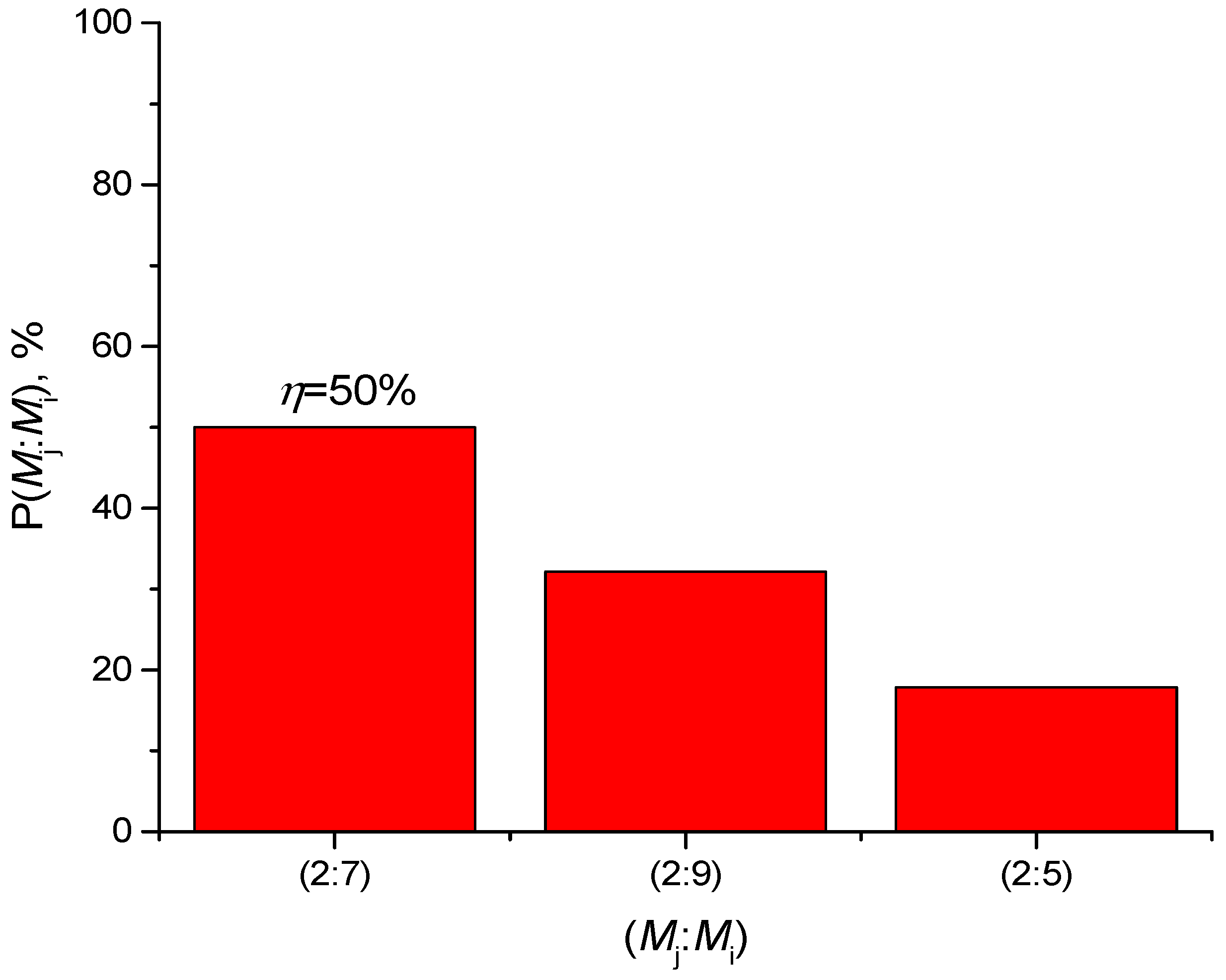
It is convenient to present the probabilities P(Mj:Mi) as a histogram where the values are positioned in the descending order of the magnitude P. For example, for the oscillogram section in Figure 7 the following histogram can be built. The histogram in Figure 8 is calculated by Formula (7), when the pairs occur the following number of times, NP(2:7) = 2, NP(2:9) = 1, NP(2:5) = 1, and the total number of periods is Ni = 28 (in real calculations, Ni was in the range of 1000–3000 for greater accuracy, see Appendix A.2).
For SHRi,j, the parameter of synchronization effectiveness η is defined as the maximum probability Pmax(Mj:Mi):
Therefore, we define the synchronization calculated above as SHRi,j = 2:7 with effectiveness of η = 50%.
The family of metrics (SHRi,j, η) allows sufficient determination of the synchronization state of two oscillators and calculation of the distance between the states, i.e., the difference between the synchronization degree. This property allows the use of metrics in an oscillator neural network training, pattern recognition systems and artificial intelligence [8,9,10,11].
Depending on the task, for example, the network training for data coding and pattern recognition, the problem of the presence or absence of synchronization SHRi,j can be solved by formally setting the synchronization effectiveness threshold ηth, so
In the majority of cases, we set ηth = 90%, meaning the signals are synchronized if 90% of their durability have a certain synchronization pattern. For the network training, this parameter can be chosen within a selected range, and it is one of the important parameters of the network adjustment [33].
The main technical problem we faced, was the problem of defining the synchronization order between the reference oscillator No.0 and the oscillator of the output layer No.10 characterized by the value SHR0,10:
The same value of SHR0,10 can be expressed in several ways: as a ratio, a simple fraction or a real number, for example, SHR0,10 = 10:3 = 10/3 = 3.33. Later, we will use this property to present the results more vividly.
Parameter SHR0,10 has the properties of an output neuron while the reference neuron may be considered as a master generator to which we calculate synchronization of other network neurons.
Two parameters SHR and η are used as the main metrics for evaluating the degree of two oscillators’ synchronization and are applied in the algorithm of ONN training.
The current oscillograms Isw(t) of oscillators No.0–10 were calculated simultaneously and contained ~250,000 points with the time interval Δt = 10µs (see Appendix A.1). Then, the oscillograms were automatically processed.
The switch parameters were unchanged in numerical simulation (see Section 2.1), while current intensities Ip_i (ION, IOFF, I0, I10), coupling strength constants s (sr, sm, so), noise amplitude Un and ηth varied.
2.4. Pattern Classifier Implementation and Problem Definition
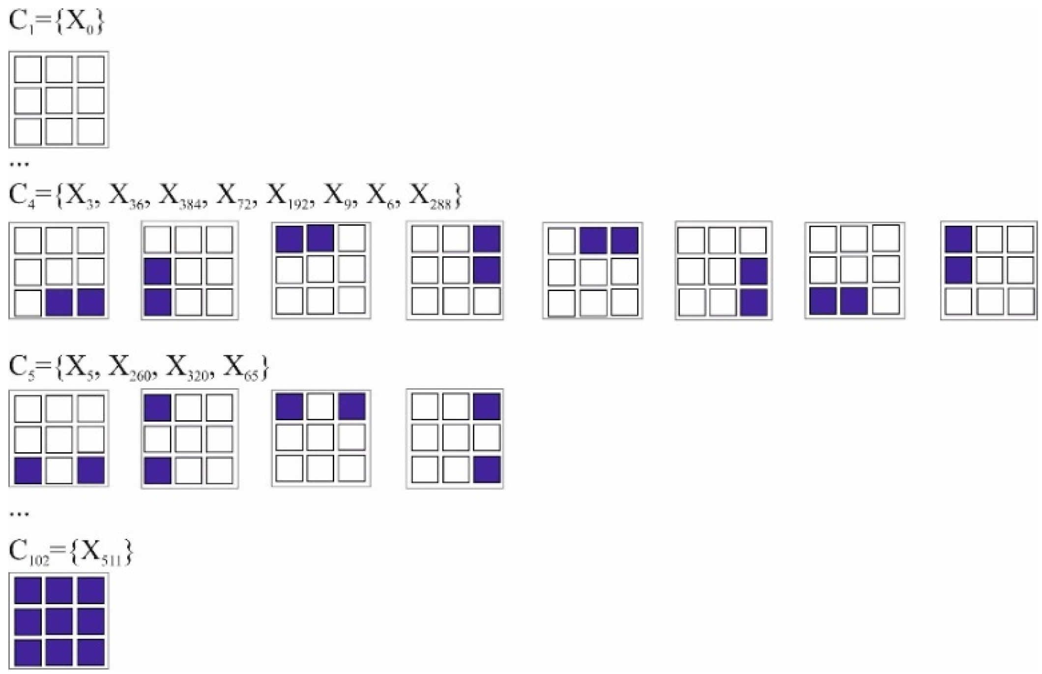
A “black-and white” pattern was used as an input test pattern presented as a 3 × 3 matrix (without gradation of gray color, 3 by 3 pixels). The form of the pattern can be unequivocally defined by the input vector Xn = (x1, …, x9) where each cell may take the value xi = 0 (white color) or xi = 1 (blue color), and n is the number of the vector equal to the decimal value of the coordinates presented as a binary sequence. For example, Figure 2 and Figure 3 show an input pattern that corresponds to the vector X489 = (1,1,1,1,0,1,0,0,1). The total number of patterns (vectors) n in the input layer matrix is 29 = 512 (X0 … X511). Presuming that the pattern processing layer together with the output layer has certain symmetry, a set of 512 vectors Xn may be divided into 102 classes Cj, where j is the number of classes (j =1 … 102) (see Figure 9). The complete list of classes and their elements is described in Supplementary Materials (Data1.txt).
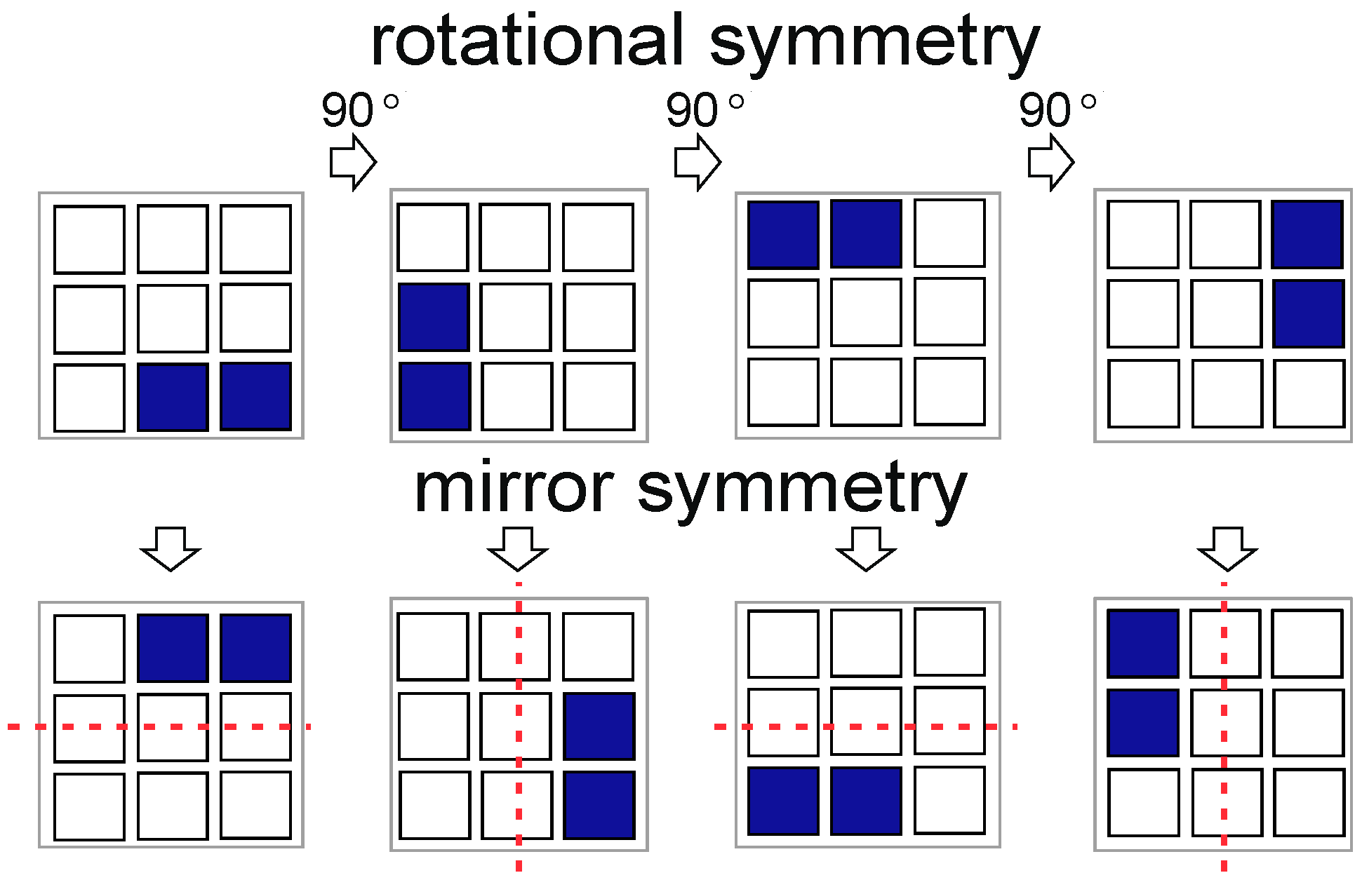
The principle of figure distribution into classes is as follows: each class Cj consists of a lot of figures (vectors) that have the same number of blue (white) cells and rotation-reflection axial symmetry of the 4th order (symmetry at rotation by 90°).
Mirror-rotation axial symmetry of the 4th order supposes an association of all figures in a separate class in the mirror operation in relation to the central columns (horizontally and vertically) and also at rotation by 90° (see the example of figures transformation for class C4 in Figure 10).
Figures from one class impose the same effect on the neural network and have the same output value SHR0,10. Distribution into classes allows us to find figures that at any current values (ION, IOFF, I0, I10) and coupling strength constants (sr, so, sm), noise amplitude Un and ηth, will have the same values of synchronization effectiveness η and SHR0,10 within one class of figures as a result of neural network symmetry. The initial distribution of all 512 figures into classes allows us to recognize not one specific figure, but a class (out of 102 possible ones) into which this figure is classified. For example, for class C5 the equality SHR0,10(X5) = SHR0,10(X260) = SHR0,10(X320) = SHR0,10(X65) will be observed.
Such classification reduces the number of possible variants to sort as we may send only 102 figures to the input layer, one figure per each class.
The problems this neural network is able to solve may be divided into several variants:
- Synchronization of oscillators No.0 and No.10 with the corresponding value of SHR0,10 and η > ηth, exists only for one specific class Cj with number j = m out of 102 classes:Here we have to show the solutions of this problem with various values of m.
- There is a set of classes C = {CZ1, CZ2 … CZP}, where Z1, Z2 … ZP are arbitrary non-repeating indices, where the number is P < 102. When inputting this set into the oscillator system, it comes to the synchronization states corresponding to the set SHR = {SHR(1)0,10, SHR(2)0,10 … SHR(P)0,10}. The set SHR does not have the same elements, i.e., each class of figures from set C corresponds to a unique synchronization order SHR0,10. By analogy with (4) the problem may be expressed as:
In fact, problem I is a subcase of problem II at P = 1.
The principle of solving problem II is shown in Figure 11. Here P = 3, and set C = {C1, C4, C5}, in this case the corresponding set is SHR = {16:15, 13:10, 14:13}. Therefore, unambiguous recognition of figures belonging to three different classes takes place. Synchronization is not realized for all other classes and η < ηth.
As there is a huge variety of set C variants, this problem can be reduced to the search of possible solutions with P > 1 and to the determination of the maximum value of P.
- III.
- The third variant of the problem corresponds to a fully trained network when it solves problem II for all possible input classes Cj, when P = 102.
In this problem, each class out of 102 possible variants corresponds to its unique value of synchronization order SHR0,10. Therefore, the set of input classes C = {C1, C2 … C102} transfers into a set of synchronous states SHR = {SHR(1)0,10, SHR(2)0,10 … SHR(102)0,10}, where all the elements have non-duplicate values.
Problems I-III have an increasing degree of complexity and are subcases of problem II with different parameter P. Problem I is the simplest one and it may be solved by a common neural network with one bistable output neuron (bistability means the presence or absence of synchronization), although two variants of answers in neural networks are often given by using two output neurons [38].
The output neuron in problems II and III have multilevel properties and differ from a common bistable neuron. All three problems can be applied to the circuit shown in Figure 2. The ONN circuit has only one output neuron, nevertheless, the multilevel high order synchronization SHR0,10 allows input pattern classification into P classes within set C. This is the most striking difference between the described neural network and variants presented in the literature. This increases the net data throughput of a single neuron and enables us to create multilevel output cascades of neural networks with high functionality.
2.5. Technique for ONN Training
To solve problems I–III, network training is required. As ONN with a high order synchronization effect has not been studied before, there are no established methods for network training. One of the ways is to use a simulated annealing algorithm [39] for the network parameters selection: current (ION, IOFF, I0, I10), coupling strength (sr, so, sm), noise amplitude Un and the synchronization effectiveness threshold ηth. The algorithm’s main point is the random searching of the problem II solution with the maximum value of P at some initial interval of parameters, followed by the narrowing of these intervals.
Determination of step size is required for direct parameter searching. In our numerical experiment, the current range was determined by the generation of oscillation in a single oscillator. For the oscillator circuit described in Section 2.1, the generation of oscillation was within the feeding current range of 550 µA ≤ Ip ≤ 1061 µA. Therefore, the currents (ION, IOFF, I0, I10) varied in this range. We determined the variation steps as δIp_i = 1 µA. So, there were 512 current steps.
For coupling strength s, the variation range was determined by the threshold values of I–V characteristics of a switch. The condition, that is, the integral thermal action on the neuron sΣ should not reduce the threshold voltage of the I–V characteristic of a switch Uth below the holding voltage Uh, must be met:
On the basis of Formula (13), for the values of threshold voltages (Uth = 5 V, Uh = 1.5 V) and coupling configurations (see Figure 2), the limits of the coupling strength variations are subject to the following conditions: (sr+ so·9) < 3.5 V and (sr+ sm·4) < 3.5 V. This condition is met with the following ranges that we have chosen: sr = 0 ÷ 0.2 V, sm = 0 ÷ 0.5 V, so = 0 ÷ 0.3 V. The variation step was chosen as 0.1% of the range magnitude.
The range 20 µV ≤ Un ≤ 900 µV with the number of steps equal to 12 was chosen for the noise amplitude.
For the synchronization effectiveness threshold ηth, the variation range was 10 % ≤ ηth < 100%, with the number of steps equal to 25 and minimal spacing δηth = 0.1%. Parameter ηth does not belong to the network parameters but rather to the parameters of the algorithm of synchronization order SHR0,10 calculation. The value ηth strongly affects the results of synchronization and the results of pattern recognition because it is a conditionally chosen characteristic. Identifying its optimal value for the recognition problems is an important step in network tuning and training.
Having a lot of network parameters, each parameter’s variant should be calculated in 102 classes together with oscillograms and synchronization values SHR0,10 at each stage. A full, direct search of all parameters’ variants would take a lot of time and computational resources. Therefore, we fixed the values Un and ηth, and varied currents (ION, IOFF, I0, I10) and couplings strength (sr, so, sm). The algorithm for searching for the solution of problem II with the maximum value P included the following steps:
Preparation step: Setting of constant values of Un and ηth
- Step 1:
- Random searching of parameters (ION, IOFF, I0, I10, sr, so, sm) in the maximal range of their variations and finding the values meeting the maximum value P. The number of searching attempts is 1000.
- Step 2:
- Narrowing of the parameters ranges by 5 times with their symmetric distribution in relation to the results of the previous step. The number of searching attempts is 1000.
- Step 3:
- Narrowing of the parameters ranges by 25 times with their symmetric distribution in relation to the results of the previous step. The number of searching attempts is 1000.
Noise amplitude Un is kept fixed because this is the parameter that is not often controlled in the experiment. It is determined by external and internal circuit noises, and we considered its effect individually in more detail. We used Un = 80 µV, which is close to the experimentally observed value [19].
The threshold value of synchronization effectiveness ηth is fixed because it is the main parameter in the synchronization algorithm, and we considered its effect individually in more detail. For the pattern recognition experiments, we used a workstation (Intel Xeon quad core processor, Albuquerque, NM, USA, 4 × 2 GHz, 8GB RAM) running 64-bit Windows Server 2008. CPU time for a single run on one core for the direct search procedure with 1000 search attempts took ~5 h.
3. Results
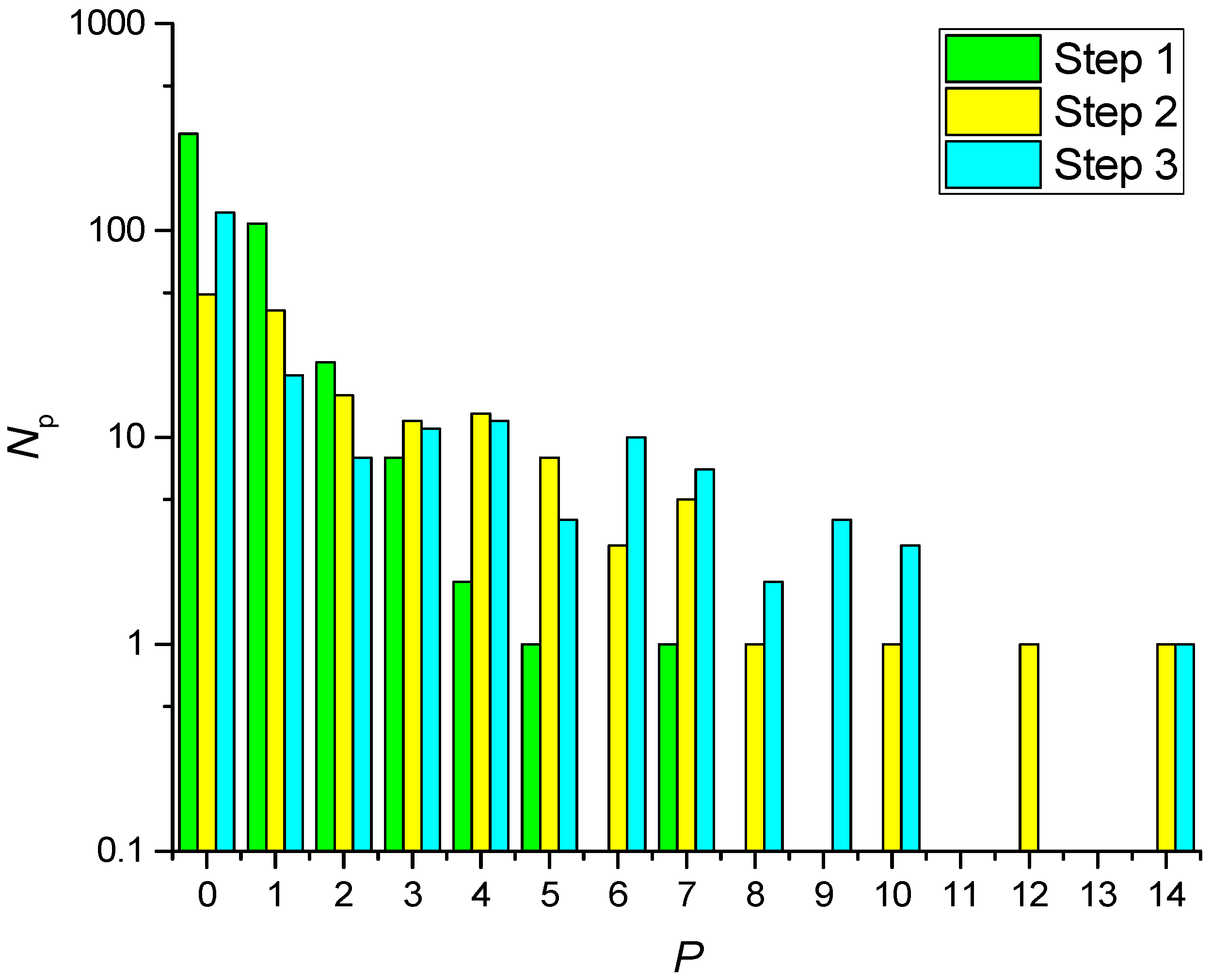
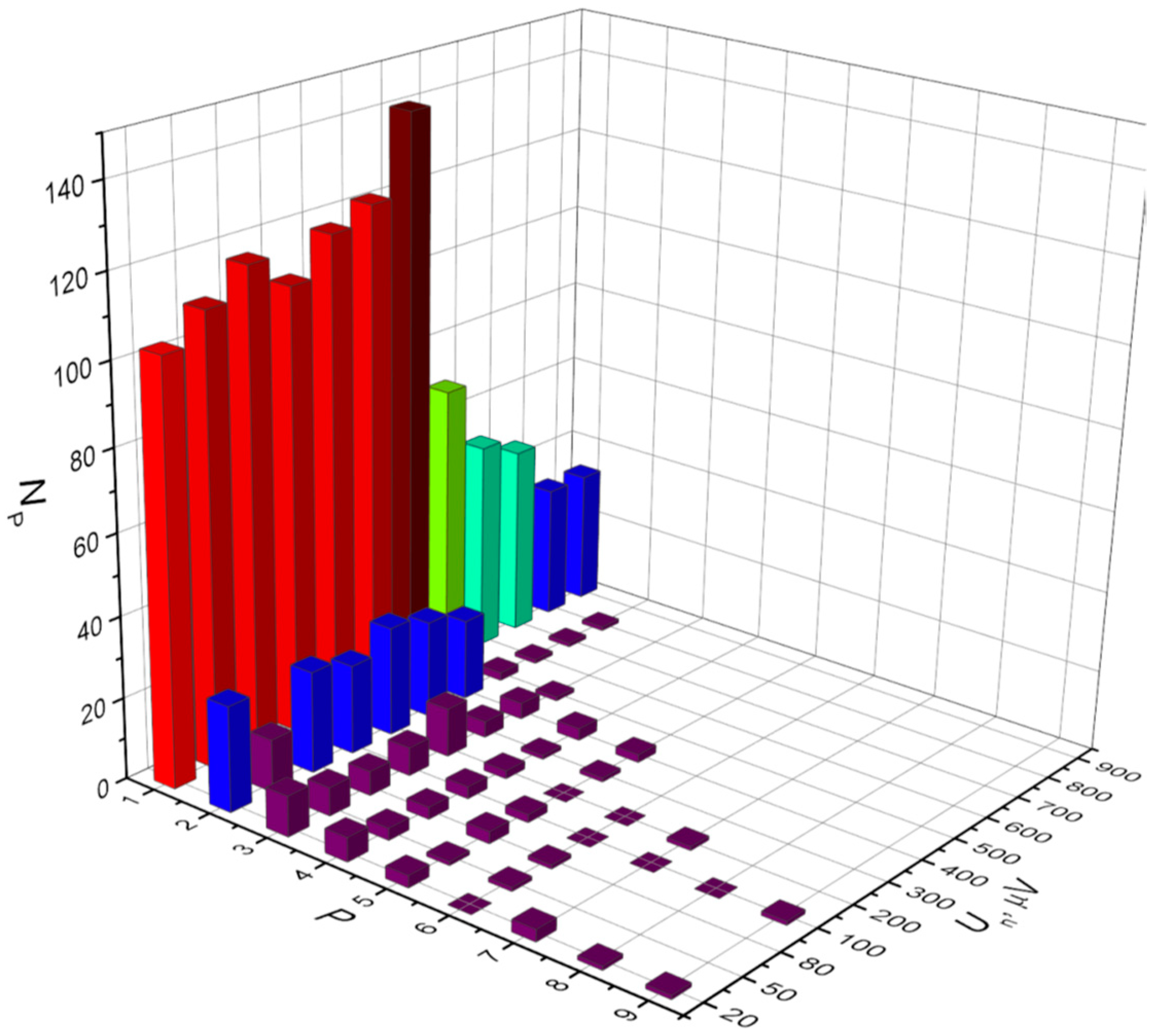
Following the proposed algorithm, we fixed the values of the following parameters (Un = 80 µV, ηth = 90%) and varied the currents (ION, IOFF, I0, I10) and coupling strength (sr, so, sm). The distribution of the solutions after the first, second and third steps of training is shown in the diagram (Figure 12), the values of P are on the x-axis, and the corresponding number of solutions NP are on the y-axis. The largest number of solutions corresponds to P = 0 when there is no synchronization at any input class Cj. After steps 2–3. the number of solutions with a low value of P decreases and the solutions with a higher value of P appear. Step 3 gives more solutions in the range P = 6–10 in comparison with step 2, although the maximum value P = 14 is similar in both cases.
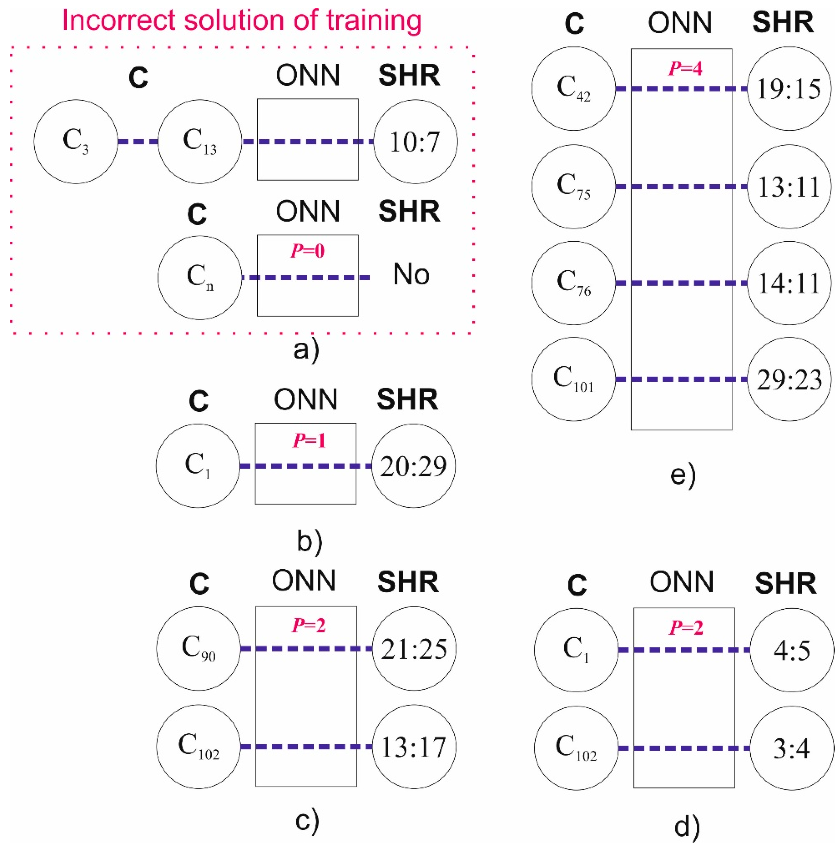
The incorrect solution of training (see Figure 13a), which does not correspond to the problem I-III conditions, occurs rather often. For example, two or more classes may correspond to the same value of SHR0,10, and the probability of such an event at the first step of training is ~55% (the calculation was based on the data in Figure 12), which results in the ambiguous recognition of figures and their classes. Another frequent case of wrong training is the absence of oscillatory synchronization for any input class (P = 0), which has a probability of ~30% in the first step (see the values in Figure 12).
3.1. Solution of Problem I
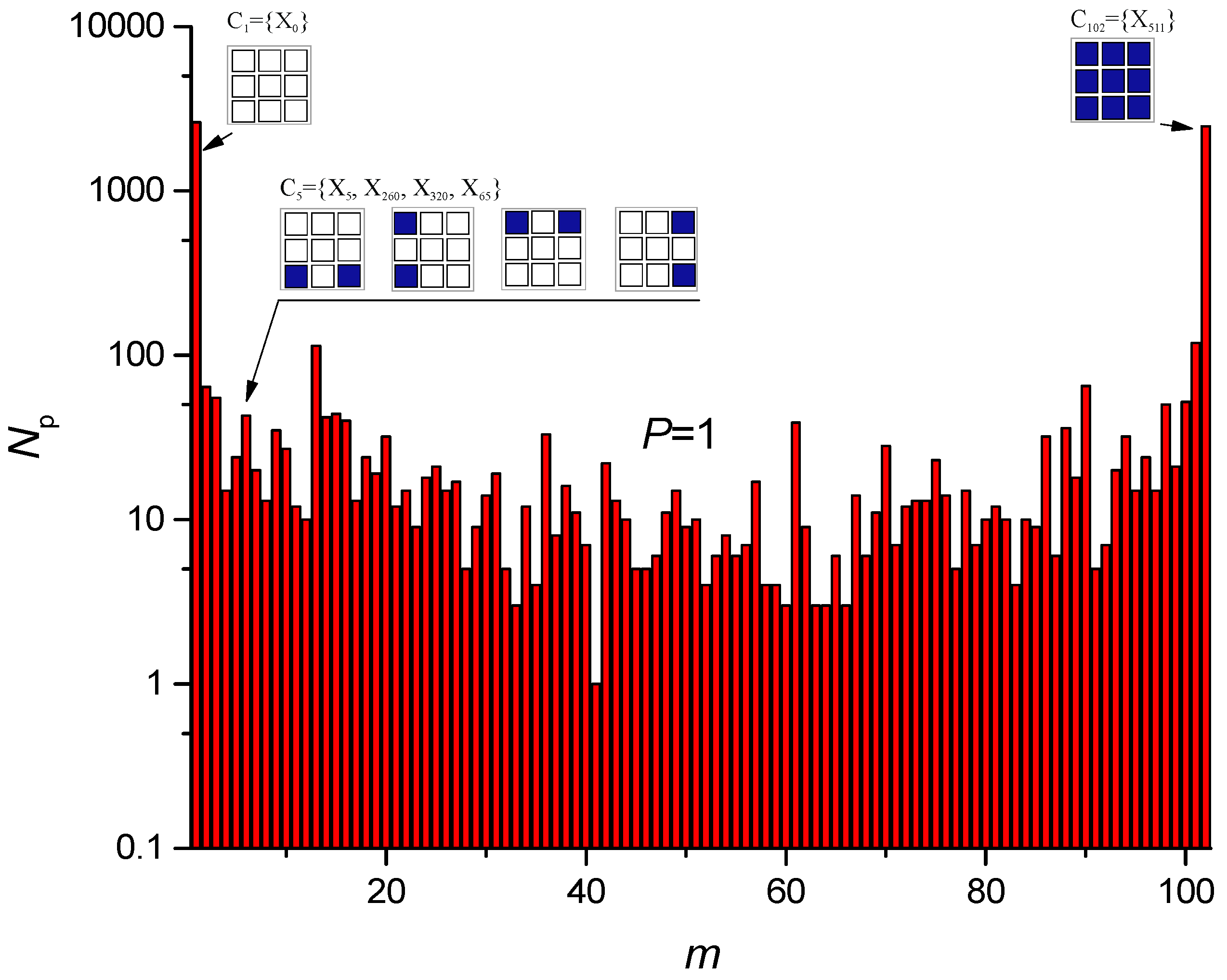
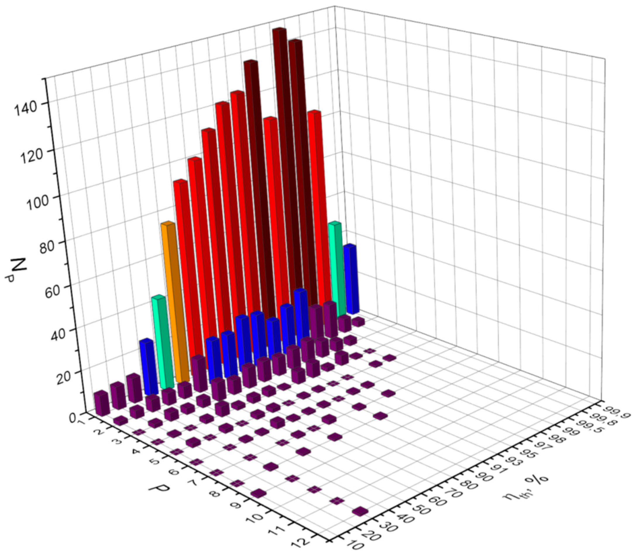
The experiment demonstrated that the solution for problem I (P = 1) is easily found for some classes Cm. For example, Figure 13b shows a neural network that recognizes class C1 with the corresponding synchronization order SHR0,10 = 20:29, and there is no synchronization for all other classes. The probability of any solution with P = 1 during the first step is ~10% (here the total number of attempts is 1000 and the value of Np ~ 100, see Figure 12), and this is the maximum probability of the solution in comparison with other P > 1. Figure 14 shows the distribution of solutions at P = 1 for various values of m (4) after 60 repetitions of the first step of training at the maximum range of all parameter variations. The maximum probability (~4%) can be seen for solutions with sets C1 and C102 when all cells of the input pattern are either empty or colored, see Figure 9. Solutions for other m are much rarer, with the probability being two orders lower (~0.03%). Parameters corresponding to the same solution can differ significantly. For example, the system can recognize class C102 at the input, while at the output SHR0,10 would be different for different parameters, however, the problem is still considered solved. The histogram shows that the network can be trained to solve problem I with a certain, predetermined value of m.
3.2. Solution of Problem II
The condition of problem II requires that a certain class from set C should correspond to the unique synchronization order from set SHR while there is no output oscillator synchronization for other classes. For example, at the first step of training, Np = 26 solutions were found for P = 2, two of them are shown in Figure 13c,d, and Figure 13e demonstrates the variant of set C and SHR for P = 4.
We can find solutions with a random search, for example, for P = 2, however, these solutions would be for different satisfying condition (12). For P = 2, there are C2102 = 5151 solution combinations (where C2102 is the number of combinations 2 out of 102). For P = 14, C14102 is a 17-digit number. Therefore, we indicate the maximum value of P, and do not indicate which solution was found.
After all training steps, the maximum value of P reached P = 14. While ONN configuration and training algorithm can be further improved, the purpose of this work is to demonstrate that a multilevel neural network can be implemented and used for pattern recognition.
3.3. Solution of Problem III
The solution for problem III has not been found yet (see Section 4).
3.4. Study of the Noise Effect on the Training Results
We constructed a 3D graph as shown in Figure 15, to find the dependence of maximum possible P and Np on the noise amplitude value in network Un (ηth = 90%). The values were taken from the first step of training.
When the noise increases above Un = 400 µV, the number of solutions NP and the value P sharply decreases. Most of the solution variants are distributed in the range 1 ≤ P ≤ 2. The maximum value for Np corresponds to P = 1 at noise level Un = 400 µV. In this case, the integral value ∑NP for all values P also has a maximum for Un = 400 µV. Therefore, “stochastic resonance” is present when a certain level of noise induces maximum number of solutions for problems I–II. This may be caused by two differently directed tendencies of Np reduction: the occurrence of “extra” synchronizations with decreasing Un and suppression of the number of synchronizations with increasing Un.
3.5. Examination of the Synchronization Threshold on the Training Result
We constructed a 3D graph as shown in Figure 16, to find the dependence of maximum possible P and Np on the value of threshold synchronization effectiveness (Un = 80 µV).
A general tendency for reduction of Np with a decrease in ηth below 40% can be seen, and the growth of ηth up to ηth = 99% on average does not change the values of P and Np. This seems to be caused by the fact that synchronization occurring during problems I and II solution has a high value of effectiveness η > 99%. In this case, reduction of ηth just adds “extra” synchronous states, which do not meet the problem conditions.
The fact that the maximum possible P reached P = 11 at ηth = 30% is interesting, and we observed some resonance for values of P. Maximum P declines as with reduction of ηth as with growth of ηth, caused by reduction of in the solution number Np.
3.6. Study of the Dynamics of the Neural Network
To understand how the output oscillator changes its synchronization relative to the reference oscillator, and what role the layer of processing neurons plays in the process, we conducted the following model experiments.
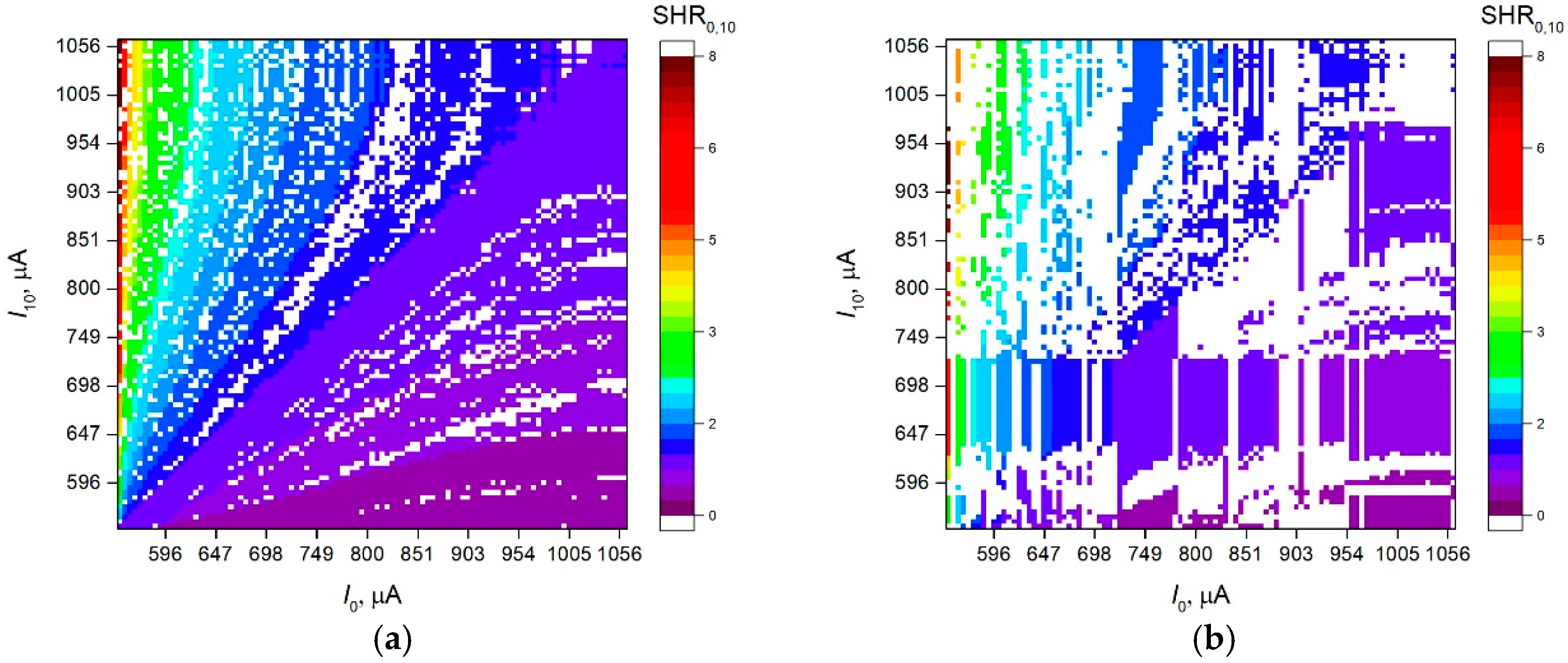
First, we turned off the effect of input oscillators on the output layer, making so = 0 V. The result was a circuit equivalent to two coupled oscillators, when oscillator No.0 affects oscillator No.10 with a force of sr = 0.3 V. By varying the oscillator currents (I0, I10), we obtained the standard distribution pattern of SHR0,10 in the form of Arnold tongue, where the regions of equal synchronization are extended sections in the form of rays (see Figure 17a) with diagonal symmetry. A special feature is a smooth (gradient) increase in SHR0,10 from the lower right distribution corner (I0 = 1061 µA, I10 = 500 µA) to the upper left corner (I0 = 500 µA, I10 = 1061 µA). Similar patterns of synchronization distribution in the system of two oscillators were observed by us earlier, for example, in [33]. After adding the effect of the processing layer, when so = 0.1 V, we get the type of synchronization distribution shown in Figure 17b. The synchronization areas are island type. The layer of input oscillators divides Arnold’s tongue into local areas while the tendency of the gradient increase in synchronization is preserved.
If we fix the currents I0 and I10, when so = 0.29 V, and vary the currents ION and IOFF, the pattern of the synchronization distribution changes its appearance (see Figure 18a). We observed a chaotic scatter of the synchronization magnitude over the field of parameters, with preservation of the diagonal symmetry and a wide scatter of values within 1–200 µA. As ION and IOFF values change the frequency of many oscillators in the processing layer at once, it is difficult to predict the tendency of the synchronization distribution. Nevertheless, the range of SHR0,10 variations is much smaller than when I0 and I10 are varied, which is obviously due to the constancy of the main frequency between the oscillators whose synchronization is measured. With a decrease in the value of so to so = 0.1 V, the form of the distribution has a similar appearance, but the range of SHR0,10 change is reduced.
In analyzing Figure 17 and Figure 18, we can assume that the model annealing method, where we randomly select the system parameters, is searching for optimal combinations of synchronization regions. Due to the large number of regions and their unpredictable order, it is possible to find a solution to problems I–II, and it is not unique, as we observed in previous experiments.
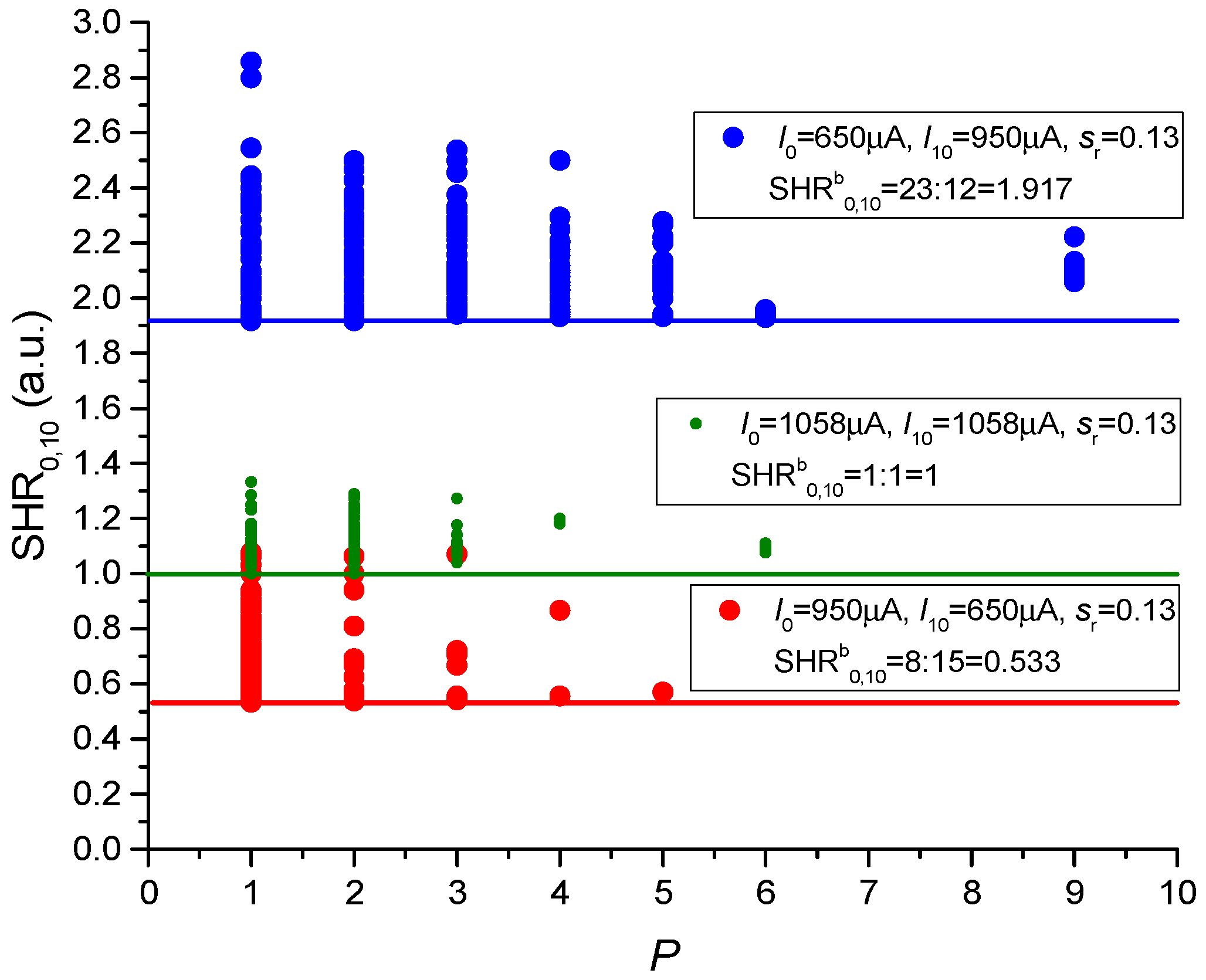
The following numerical experiment shows some features of the network operation dynamics. The idea was to find out how the matrix of the processing layer affects the synchronization of oscillators No.0 and No.10. Let us consider two cases. In the first case, so = 0 V, sr = 0.13 V, I0 = 650 µA, I10 = 950 µA, there is only one unidirectional effect of oscillator No.0 on No.10, and the base synchronization has the value SHRb0,10 = 23:12 = 1.917. In the second case, we added random variations of coupling strength (so, sm) and currents (ION, IOFF) at the same values of sr = 0.13, I0 = 650 µA, I10 = 950 µA. As a result, after the first step of training we obtained a set of solutions (C and SHR) for various P > 0 and positioned all elements of SHR0,10 on the plot (see Figure 19). It can be seen that all elements of the sets SHR are distributed within some interval above the boundary SHRb0,10. The dispersion is δSHR0,10 ~0.6.
The same behavior is observed when the current values were interchanged (I0 = 950 µA and I10 = 650 µA). The base synchronization had the value of SHRb0,10 = 8:15 = 0.533, and when other parameters were varied, the elements of SHR diverge upward with δSHR0,10 ~ 0.4. At high and similar values of current I0 = 1058 µA and I10 = 1058 µA, the base synchronization is SHRb0,10 = 1:1 = 1, and δSHR0,10 ~ 0.3.
Thus, the matrix of processing layer oscillators only deviates the SHR0,10 value upward from the base synchronization value of oscillators No.0 and No.10. The effect of oscillators positioned in the processing layer only increases the frequency of oscillator No.10, but cannot decrease it because of the nature of thermal coupling, which can initiate switching but cannot suppress it.
4. Discussion
In the previous section, we demonstrated how the simulated annealing algorithm can be used for ONN training. In this algorithm, we used three steps for parameter searching, however, we did not manage to surpass the maximum value of P = 14 (see Figure 12). Therefore, we can assume that the simulated annealing method reaches a solution limit, and to search the network parameters with higher P, it might be necessary to vary other ONN properties, for example, the number of oscillators of the processing layer, the I–V characteristics of oscillators, and the matrix of couplings S. Furthermore, the values of Un could be selected more carefully on the basis of the regularities shown in Figure 15, where the maximum of the solution number NP at a certain noise level is presented. This effect is similar to stochastic resonance phenomena in spike networks [40,41,42], and requires additional research and analysis.
The simulated annealing algorithm might not be an effective training method, and development of more efficient algorithms for this type of network is a separate global problem for future research.
For proper network training, a deeper understanding of the physics of the oscillators’ synchronization process is necessary. For example, the results and regularities arising in Figure 19 assist in understanding the process of solution generation. We demonstrated the presence of a boundary for SHR values that is determined by the base synchronization value SHRb0,10 of oscillators No.0 and No.10 and showed that the effect of oscillators’ processing layer leads to SHR0,10 ≥ SHRb0. The selection of currents for the reference oscillators No.0 and No.10 determines the variation range of δSHR0,10, and most likely, the larger this range is, the higher the probability of finding the solutions with high P. If we set the current values I0, I10, for example, at the boundary of the maximum range I0 = 1058 µA, I10 = 1058 µA, then it will be more difficult for the matrix of oscillators in the processing layer to change the dynamics of the output oscillator that operates in a high frequency mode and under the high frequency effect of the reference oscillator. As a result, we observed narrowing of δSHR0,10 to ~0.3 (see Figure 19). Figure 18 demonstrates the areas of parameters where SHR0,10 practically does not change and where it changes very often, therefore, this may explain the productivity of the annealing training algorithm. In Step 1, we found areas with a large number of solutions, and then in Step 2 and 3, by thorough scanning of these areas, we found solutions with the largest P (see Figure 12).
In addition to the configuration and network parameters, the selection of parameter ηth, which is used in the synchronization magnitude determination method, is of great importance. As the results and regularities arising in Figure 16 show, too high (ηth ≥ 99.8) and too low (ηth ≤ 20) parameters significantly reduce the number of solutions NP. Nevertheless, we suppose that the usage of ηth < 50% is not completely justified, as the parameter η determines the share of a synchronous signal in the total oscillogram [19]. Moreover, the technique of SHR determination may affect the result, and future research aimed at its improvement may lead to positive shifts in this field. The addition of alternative methods of pattern transfer into a network that vary, for example, current I10 or couplings magnitudes may significantly expand the range of variations of SHR0,10, hence, the maximal attainable value P.
The network structure defined by the coupling matrix S (1) was chosen in order to implement an actual VO2–based device, therefore, oscillator No.0 affected all other oscillators. This can be easily implemented by arranging VO2-switches on one substrate. Nevertheless, the development of an actual device requires specific setting of coupling strengths that depend on many parameters [19] and this is beyond the scope of the current work.
Although problem III has not been solved, the presented results and solution for problem II for P = 14 showed that multilevel high order synchronization increases net data throughput of a single neuron and enables the creation of multilevel output cascades of neural networks with high functionality.
The duration of the processed oscillograms was ~2.5 s (for the number of pulses ~3000), providing an error less than 0.2% for calculating η (see Appendix A.2). In the experiment, such duration would significantly slow down the work with the system, since the time of the synchronization calculation would be several seconds. Nevertheless, we hope for a real implementation of this idea on oscillators with a large generation frequency (~ 1–10 MHz), which would significantly reduce the oscillogram duration and the time for the synchronization calculation.
5. Conclusions
The paper presents a new model of ONN with high order harmonics synchronization that recognizes and classifies visual patterns by unique synchronous states, i.e., in accordance with their definite symmetry class. The most outstanding feature of this neural network, in comparison with published variants, is that neurons possess not only bistable properties (the presence or absence of synchronization with the reference neuron) but exhibit multilevel synchronization. The presented model has only one output neuron, nevertheless, variation in the value of high order synchronization SHR0,10 allows its usage to classify the input pattern into P classes with the set C. The training implementation of this network for solving cognitive tasks is an interesting possibility, as the network consists only of oscillators and does not use other computational modules.
The main purpose of the article was to demonstrate a new method of pattern recognition based on coupled oscillators, where cognitive functions are realized due to the high order synchronization effect. This is a universal effect, so regardless of the type of connection, thermal or any other, the cognitive functions can be realized using coupled oscillators. Thermal communication has no special role in pattern recognition, it is only necessary for organizing the synchronization of oscillators.
The development of ONN models with high order synchronization effect offers significant potential for increasing the efficiency of artificial intelligence networks, and the development of their training techniques is an important direction for further research. The possibility of implementing this ONN as not only a program code but also as a separately operating device based on real micro- and nano-electronic self-oscillators would enhance the importance of the obtained results and promote further research in this field.
Supplementary Materials
The following are available online at https://www.mdpi.com/2079-9292/8/1/75/s1, list of classes: Data1.txt, Data2.txt.
Author Contributions
Conceptualization, A.V.; methodology, A.V., M.B. and P.B.; software, A.V.; validation, P.B.; writing—original draft preparation, A.V., M.B. and P.B.; project administration, A.V.
Funding
This research was supported by the Russian Science Foundation (grant no. 16-19-00135).
Acknowledgments
The authors express their gratitude to O. Dobrynina and Andrei Rikkiev for the valuable comments in the course of the article translation and revision.
Conflicts of Interest
The authors declare no conflict of interest.
Appendix A
Appendix A.1. Model Circuit of a Coupled Oscillators-Based Neural Network
The circuit of the modelled ONN is presented in Figure 2. It consists of 11 oscillators numbered i = 0 … 10. The magnitude of the i-th oscillator effect on the j-th oscillator is determined by the coupling strength si,j, which is set by matrix S (1).
The model circuit of a single oscillator is given in Figure A1. It includes a source of current Ip_i, capacitance C connected in parallel with a VO2 switch and noise source Un_i. The capacity magnitude C was constant C = 1 00 nF, but Ip_i and Un_i varied within the following ranges: Ip (550 µA ÷ 1061 µA), Un (20 µV ÷ 900 µV). The current through the VO2 switch and its voltage are defined as Isw_i and Ui, respectively. Voltage-current characteristics of the VO2 switch are shown in Figure A2, where the experimental and model curves are presented.
Figure A1.
Circuit of a single oscillator of a VO2-based structure. I is the number of an oscillator; Ip_i is a source of current, C is a capacitance, Un_i is a source of noise, Isw_i is the current through the VO2 switch, Ui is the voltage at the switch.
Figure A1.
Circuit of a single oscillator of a VO2-based structure. I is the number of an oscillator; Ip_i is a source of current, C is a capacitance, Un_i is a source of noise, Isw_i is the current through the VO2 switch, Ui is the voltage at the switch.

Figure A2.
Typical experimental I–V characteristics of a separate switch (Experiment curve) and its model curve (Model curve).
Figure A2.
Typical experimental I–V characteristics of a separate switch (Experiment curve) and its model curve (Model curve).

All model switches without coupling have the same I–V characteristics, with stationary natural parameters Uth = 5 V (threshold voltage), Uh = 1.5 V (holder voltage), Ucf = 0.82 V (cutoff voltage).
The model curve Isw_i = f(Ui), which has high-resistance (OFF) and low-resistance (ON) segments with corresponding dynamic resistances Roff_i = 9100 Ω and Ron_i = 615 Ω, can be presented by the following formula:
where i = 0 … 10 is the oscillator number, flagi denotes the VO2 switch state 1 (OFF—high resistance), 0 (ON—low resistance).
Transitions from one state into another can be expressed by the following algorithm:
where Uth_i and Uh_i are threshold turn-on and holder voltages of switches (see Figure A3):
As mentioned in Section 2.1, the model of thermal coupling is based on reduction of threshold voltage Uth by the value s due to thermal effect of other switches. The value s is the thermal coupling strength. The physics of thermal interaction is caused by the generation of a heat wave when the switch is turned on, which propagates and acts (heats) on the surrounding switching structures. In [19], we showed that it is possible to introduce an interaction radius RTC beyond which the induced temperature is less than 0.2 K. Therefore, in the model, we assume that each switch only interacts with surrounding switches that are within the radius of RTC. The heating of structures leads to a decrease in the threshold voltage [19], this change characterizes the value of s, which we call the coupling force. The higher the s, the stronger the effect of one switch on the other.
Coupling of oscillators results in changing their threshold turn-on voltages Uth_i in regard to the switch state (flagi) with which they interact.
In general, the magnitude Uth i can be presented by the following formula:
where j runs though all values, at which the switch is in turn-on state (flagi = 0), and Uth is the natural turn-on voltage without coupling.
This means that all effects of sj,i on i-switch are summed up from all the other j-th switches at the turn-on state.
The differential equation that describes the circuit operation (Figure A2) is written as:
where I is the number of an oscillator, C is capacitance, Uc_i is the capacitor voltage, Isw_i is the current through the switch, Un_i is the noise in the switch, and f(U) is the I–V characteristic function (A1).
Equations (A4) were numerically calculated with respect to time at regular intervals Δt = 10−5 s using implicit Euler method and discrete noise Un(t) was generated according to the algorithm Un(t) = Un0·randn(t), where Un0—noise amplitude and randn(t)—normal random numbers generated with zero mean and dispersion equal to 1, realized through the algorithm of uniformly distributed random value transformation [43].
As a result, by setting oscillator current values Ip_i, noise amplitude Un0, and coupling strengths (sr, sm, so) we could calculate oscillograms of current Isw_i(t), voltage at the capacity Uc_i(t) and voltage at switches:
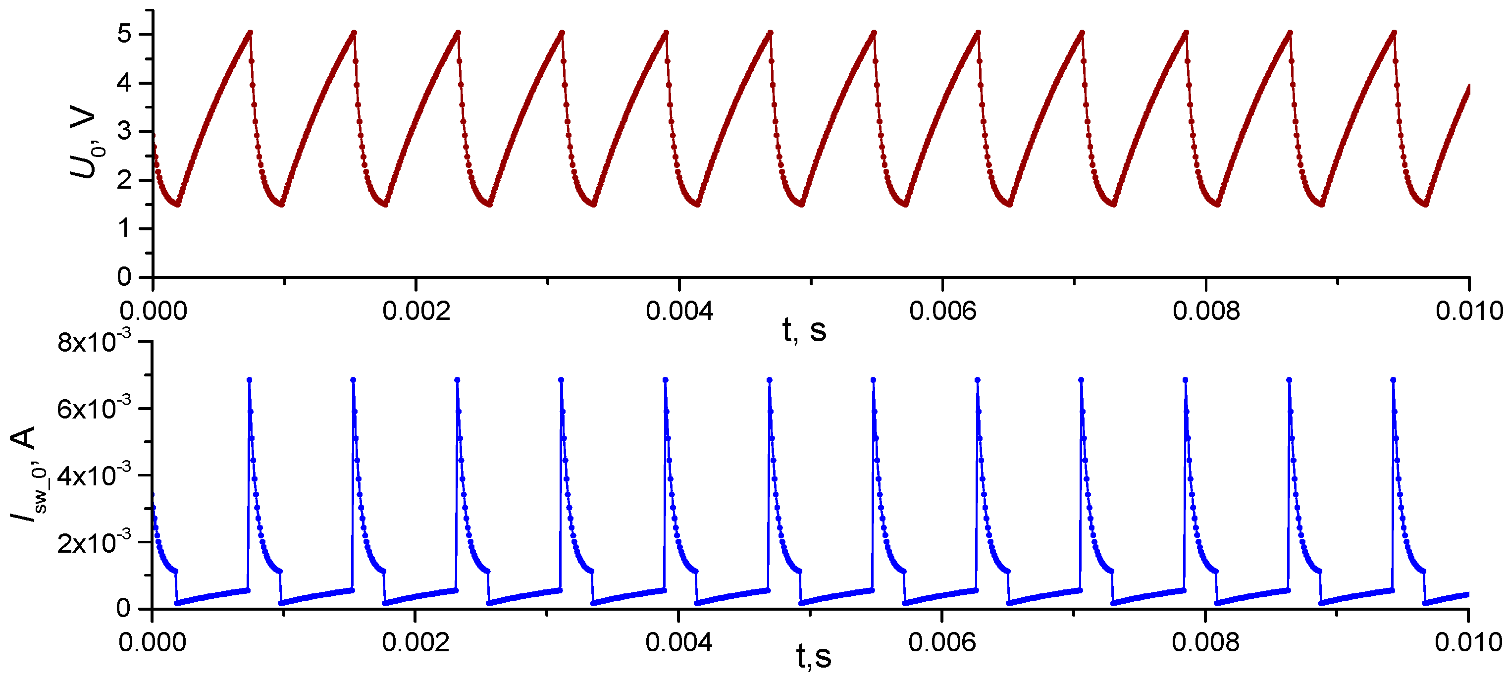
Figure A3.
Examples of calculated oscillograms sections (1000 points), voltage U0 and current Isw_0, for the oscillator with i = 0 at Ip_0 = 1200 µA. Here we do not show other circuit parameters because other oscillators do not affect this one.
Figure A3.
Examples of calculated oscillograms sections (1000 points), voltage U0 and current Isw_0, for the oscillator with i = 0 at Ip_0 = 1200 µA. Here we do not show other circuit parameters because other oscillators do not affect this one.

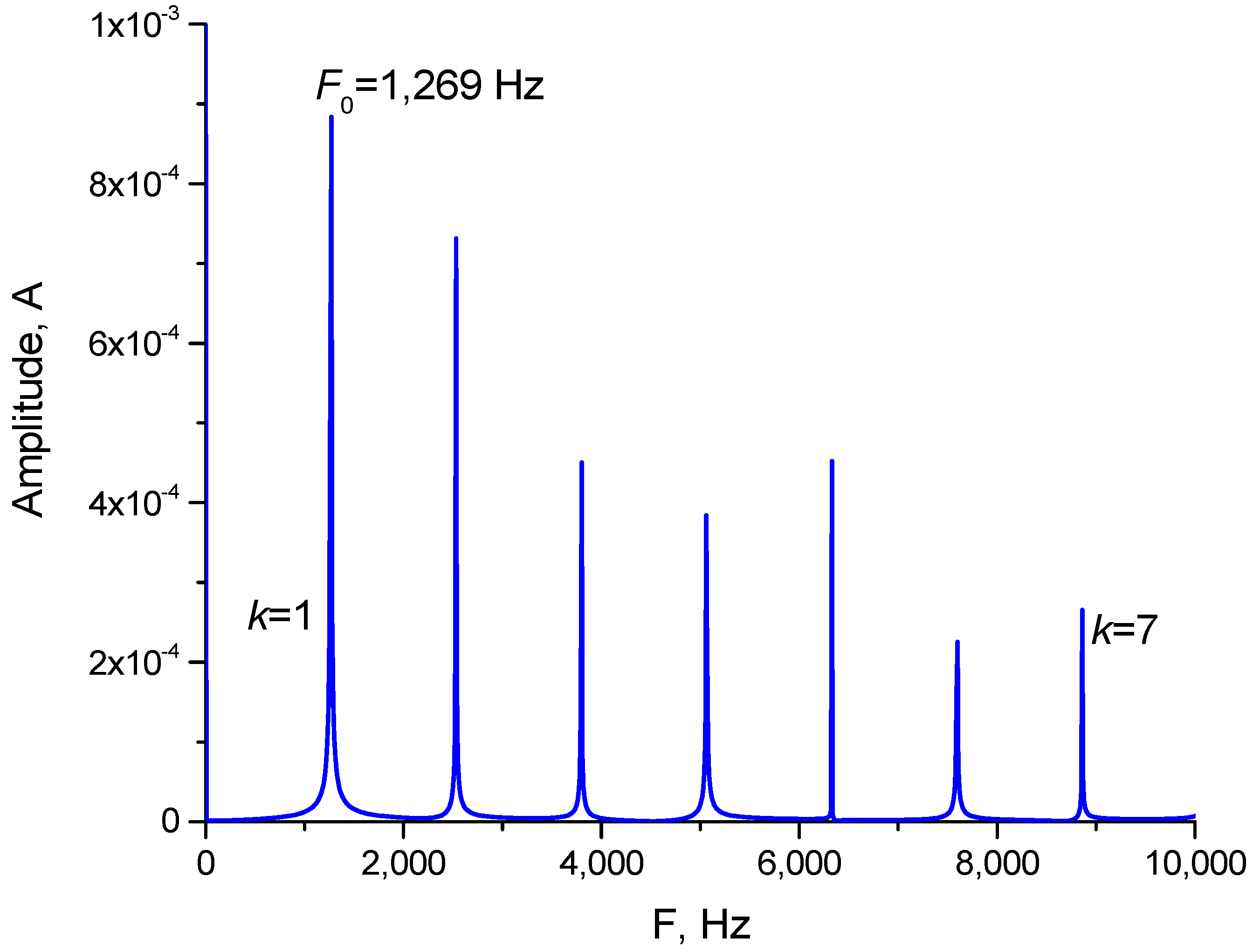
Figure A4.
Spectrum of a current signal for the oscillogram shown in Figure A3.
Figure A4.
Spectrum of a current signal for the oscillogram shown in Figure A3.

Examples of sections (1000 points) of calculated oscillograms for voltage U0 and current Isw_0 are shown in Figure A3. The spectrum of the current signal has a large number of harmonics, see Figure A4. The main frequency F0 = 1269 Hz determines the period of current oscillations T0 ~ 788 µs (because T0 = 1/F0).
The interaction between the oscillators occurs according to the current signal as it is shown in the model, and has also been observed in an actual experiment, see [19,35], because the current signal is transformed into thermal pulses that spread along the substrate. As a result, the high order synchronization effect can be observed between the coupled oscillators.
Appendix A.2. Dependence of SHR0,10 and η on the Number of Pulses in the Oscillogram
An important issue in calculating SHR0,10 and η according to the method in Section 2.3, with the desired accuracy, is the determination of the number of pulses used for the calculation. In fact, it is necessary to set the minimum duration of the processed oscillogram. This is also important for determining the minimum calculation time for a family of metrics. For example, in a real experiment to calculate SHR0,10 and η, it is required to record the oscillogram, and then make the calculation. In a model experiment, this time is determined by the oscillogram simulation time.
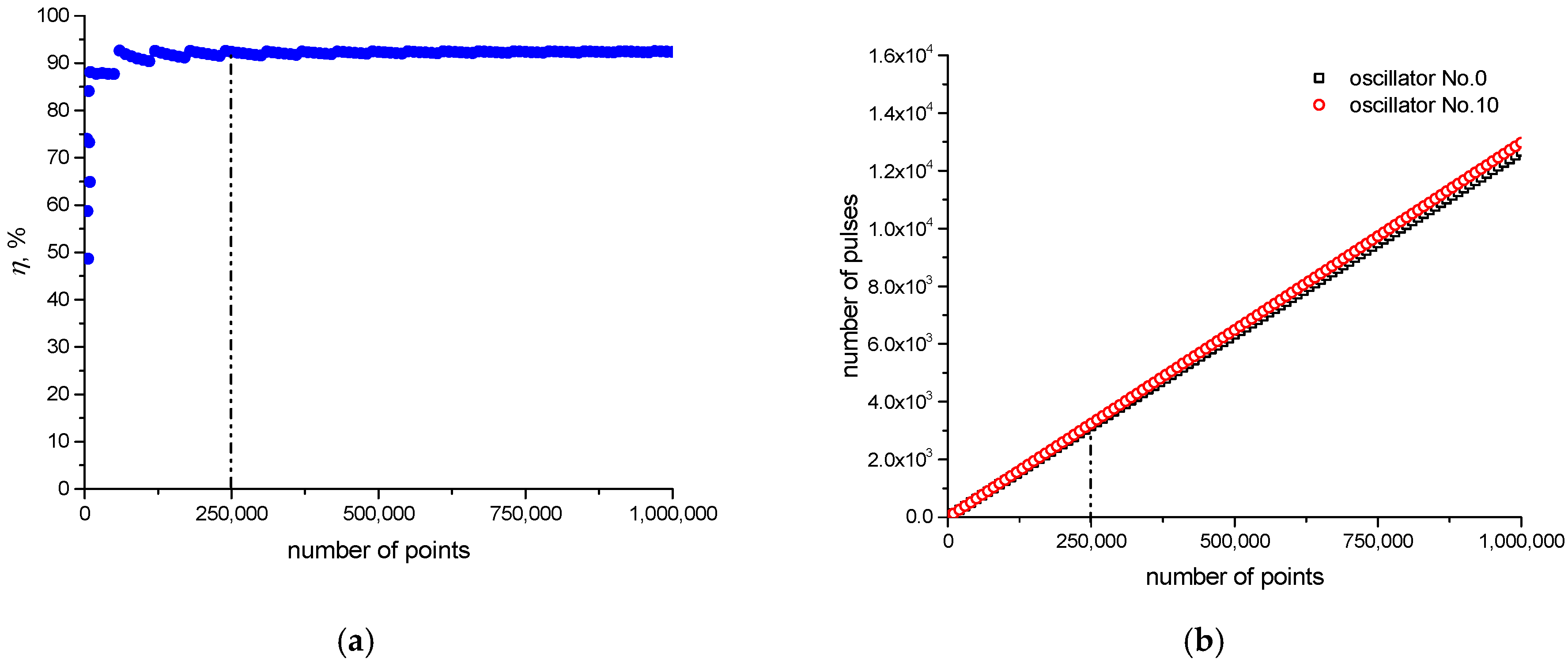
Figure A5a shows the dependence of η on the number of oscillogram points with the following system parameters (I0 = 1017 µA, I10 = 891 µA, ION = 725 µA, IOFF = 1035 µA sr = 0.1036 V, sm = 0.207 V, so = 0.29298 V, ηth=90%, Un = 80 µV, the input image is X3). With an increase in the number of points, the number of pulses in the oscillograms of oscillators No.0 and No.10 grows (see Figure A5b.)
Figure A5.
The dependence of η (a) and the number of pulses (b) on the number of points on the oscillogram. The dashed line corresponds to 250,000 oscillogram points.
Figure A5.
The dependence of η (a) and the number of pulses (b) on the number of points on the oscillogram. The dashed line corresponds to 250,000 oscillogram points.

With an increase in the number of points (pulses) in the processed oscillogram, the value of η comes to saturation, which is the true value of η. The synchronization value is defined as SHR0.10 = 38:37 with the number of points more than 60,000 (when η ≥ ηth at ηth = 90%); with a smaller number of points, the synchronization is not detected (η < ηth).
In this work, we used 250,000 points (the number of pulses ~3000), which gives an error less than 0.2% in determining η. The duration of the oscillogram was ~2.5 s (Δt = 10−5 s).
References
- Freeman, W.J. Spatial properties of an EEG event in the olfactory bulb and cortex. Electroencephalogr. Clin. Neurophysiol. 1978, 44, 586–605. [Google Scholar] [CrossRef]
- Von der Malsburg, C. The Correlation Theory of Brain Function. In Models of Neural Networks; Springer: New York, NY, USA, 1994; pp. 95–119. [Google Scholar] [Green Version]
- Gray, C.M.; Singer, W. Stimulus-specific neuronal oscillations in orientation columns of cat visual cortex. Proc. Natl. Acad. Sci. USA 1989, 86, 1698–1702. [Google Scholar] [CrossRef] [PubMed]
- Eckhorn, R.; Bauer, R.; Jordan, W.; Brosch, M.; Kruse, W.; Munk, M.; Reitboeck, H.J. Coherent oscillations: A mechanism of feature linking in the visual cortex? Biol. Cybern. 1988, 60, 121–130. [Google Scholar] [CrossRef] [PubMed]
- Burton, S.D.; Ermentrout, G.B.; Urban, N.N. Intrinsic heterogeneity in oscillatory dynamics limits correlation-induced neural synchronization. J. Neurophysiol. 2012, 108, 2115–2133. [Google Scholar] [CrossRef] [PubMed] [Green Version]
- White, J.A.; Chow, C.C.; Rit, J.; Soto-Treviño, C.; Kopell, N. Synchronization and Oscillatory Dynamics in Heterogeneous, Mutually Inhibited Neurons. J. Comput. Neurosci. 1998, 5, 5–16. [Google Scholar] [CrossRef] [PubMed]
- Akam, T.; Kullmann, D.M. Oscillations and Filtering Networks Support Flexible Routing of Information. Neuron 2010, 67, 308–320. [Google Scholar] [CrossRef] [PubMed] [Green Version]
- Kuzmina, M.; Manykin, E.; Surina, I. Oscillatory network with self-organized dynamical connections for synchronization-based image segmentation. Biosystems 2004, 76, 43–53. [Google Scholar] [CrossRef]
- Corinto, F.; Bonnin, M.; Gilli, M. Weakly Connected Oscillatory Network Models for Associative and Dynamic Memories. Int. J. Bifurc. Chaos 2007, 17, 4365–4379. [Google Scholar] [CrossRef]
- Nikonov, D.E.; Csaba, G.; Porod, W.; Shibata, T.; Voils, D.; Hammerstrom, D.; Young, I.A.; Bourianoff, G.I. Coupled-Oscillator Associative Memory Array Operation for Pattern Recognition. IEEE J. Explor. Solid-State Comput. Devices Circuits 2015, 1, 85–93. [Google Scholar] [CrossRef]
- Hoppensteadt, F.C.; Izhikevich, E.M. Pattern recognition via synchronization in phase-locked loop neural networks. IEEE Trans. Neural Netw. 2000, 11, 734–738. [Google Scholar] [CrossRef] [Green Version]
- Acebrón, J.A.; Bonilla, L.L.; Pérez Vicente, C.J.; Ritort, F.; Spigler, R. The Kuramoto model: A simple paradigm for synchronization phenomena. Rev. Mod. Phys. 2005, 77, 137–185. [Google Scholar] [CrossRef] [Green Version]
- Klinshov, V.V.; Nekorkin, V.I. Synchronization of delay-coupled oscillator networks. Physics-Uspekhi 2013, 56, 1217–1229. [Google Scholar] [CrossRef]
- Vassilieva, E.; Pinto, G.; Acacio de Barros, J.; Suppes, P. Learning Pattern Recognition Through Quasi-Synchronization of Phase Oscillators. IEEE Trans. Neural Netw. 2011, 22, 84–95. [Google Scholar] [CrossRef] [PubMed] [Green Version]
- Hagerstrom, A.M.; Murphy, T.E.; Roy, R.; Hövel, P.; Omelchenko, I.; Schöll, E. Experimental observation of chimeras in coupled-map lattices. Nat. Phys. 2012, 8, 658–661. [Google Scholar] [CrossRef] [Green Version]
- Vodenicarevic, D.; Locatelli, N.; Abreu Araujo, F.; Grollier, J.; Querlioz, D. A Nanotechnology-Ready Computing Scheme based on a Weakly Coupled Oscillator Network. Sci. Rep. 2017, 7, 44772. [Google Scholar] [CrossRef] [Green Version]
- Romera, M.; Talatchian, P.; Tsunegi, S.; Abreu Araujo, F.; Cros, V.; Bortolotti, P.; Trastoy, J.; Yakushiji, K.; Fukushima, A.; Kubota, H.; et al. Vowel recognition with four coupled spin-torque nano-oscillators. Nature 2018, 563, 230–234. [Google Scholar] [CrossRef]
- Pikovsky, A.; Rosenblum, M.; Kurths, J. Synchronization: A Universal Concept in Nonlinear Sciences; Cambridge University Press: Cambridge, UK, 2001; ISBN 9780521533522. [Google Scholar]
- Velichko, A.; Belyaev, M.; Putrolaynen, V.; Perminov, V.; Pergament, A. Thermal coupling and effect of subharmonic synchronization in a system of two VO2 based oscillators. Solid-State Electron. 2018, 141, 40–49. [Google Scholar] [CrossRef]
- Sakai, J. High-efficiency voltage oscillation in VO2 planer-type junctions with infinite negative differential resistance. J. Appl. Phys. 2008, 103, 103708. [Google Scholar] [CrossRef]
- Shukla, N.; Parihar, A.; Freeman, E.; Paik, H.; Stone, G.; Narayanan, V.; Wen, H.; Cai, Z.; Gopalan, V.; Engel-Herbert, R.; et al. Synchronized charge oscillations in correlated electron systems. Sci. Rep. 2015, 4, 4964. [Google Scholar] [CrossRef]
- Maffezzoni, P.; Daniel, L.; Shukla, N.; Datta, S.; Raychowdhury, A. Modeling and Simulation of Vanadium Dioxide Relaxation Oscillators. IEEE Trans. Circuits Syst. I Regul. Pap. 2015, 62, 2207–2215. [Google Scholar] [CrossRef] [Green Version]
- Belyaev, M.A.; Boriskov, P.P.; Velichko, A.A.; Pergament, A.L.; Putrolainen, V.V.; Ryabokon, D.V.; Stefanovich, G.B.; Sysun, V.I.; Khanin, S.D. Switching Channel Development Dynamics in Planar Structures on the Basis of Vanadium Dioxide. Phys. Solid State 2018, 60, 447–456. [Google Scholar] [CrossRef]
- Boriskov, P.P.; Velichko, A.A.; Pergament, A.L.; Stefanovich, G.B.; Stefanovich, D.G. The effect of electric field on metal-insulator phase transition in vanadium dioxide. Tech. Phys. Lett. 2002, 28, 406–408. [Google Scholar] [CrossRef]
- Datta, S.; Shukla, N.; Cotter, M.; Parihar, A.; Raychowdhury, A. Neuro Inspired Computing with Coupled Relaxation Oscillators. In Proceedings of the 51st Annual Design Automation Conference on Design Automation Conference—DAC ’14; ACM Press: New York, NY, USA, 2014; pp. 1–6. [Google Scholar]
- Parihar, A.; Shukla, N.; Datta, S.; Raychowdhury, A. Exploiting Synchronization Properties of Correlated Electron Devices in a Non-Boolean Computing Fabric for Template Matching. IEEE J. Emerg. Sel. Top. Circuits Syst. 2014, 4, 450–459. [Google Scholar] [CrossRef]
- Shukla, N.; Parihar, A.; Cotter, M.; Barth, M.; Li, X.; Chandramoorthy, N.; Paik, H.; Schlom, D.G.; Narayanan, V.; Raychowdhury, A.; et al. Pairwise coupled hybrid vanadium dioxide-MOSFET (HVFET) oscillators for non-boolean associative computing. In 2014 IEEE International Electron Devices Meeting; IEEE: San Francisco, CA, USA, 2014; pp. 28.7.1–28.7.4. [Google Scholar]
- Velichko, A.; Belyaev, M.; Putrolaynen, V.; Pergament, A.; Perminov, V. Switching dynamics of single and coupled VO2-based oscillators as elements of neural networks. Int. J. Mod. Phys. B 2017, 31, 1650261. [Google Scholar] [CrossRef]
- Ghosh, S. Generation of high-frequency power oscillation by astable mode arcing with SCR switched inductor. IEEE J. Solid-State Circuits 1984, 19, 269–271. [Google Scholar] [CrossRef]
- Chen, C.L.; Mathews, R.H.; Mahoney, L.J.; Calawa, S.D.; Sage, J.P.; Molvar, K.M.; Parker, C.D.; Maki, P.A.; Sollner, T.C.L.G. Resonant-tunneling-diode relaxation oscillator. Solid-State Electron. 2000, 44, 1853–1856. [Google Scholar] [CrossRef]
- Sharma, A.A.; Bain, J.A.; Weldon, J.A. Phase Coupling and Control of Oxide-Based Oscillators for Neuromorphic Computing. IEEE J. Explor. Solid-State Comput. Devices Circuits 2015, 1, 58–66. [Google Scholar] [CrossRef]
- Locatelli, N.; Cros, V.; Grollier, J. Spin-torque building blocks. Nat. Mater. 2014, 13, 11–20. [Google Scholar] [CrossRef] [Green Version]
- Velichko, A.; Belyaev, M.; Putrolaynen, V.; Boriskov, P. New Method of the Pattern Storage and Recognition in Oscillatory Neural Networks Based on Resistive Switches. Electronics 2018, 7, 266. [Google Scholar] [CrossRef]
- Velichko, A.A.; Stefanovich, G.B.; Pergament, A.L.; Boriskov, P.P. Deterministic noise in vanadium dioxide based structures. Tech. Phys. Lett. 2003, 29, 435–437. [Google Scholar] [CrossRef]
- Velichko, A.; Belyaev, M.; Putrolaynen, V.; Perminov, V.; Pergament, A. Modeling of thermal coupling in VO2-based oscillatory neural networks. Solid-State Electron. 2018, 139, 8–14. [Google Scholar] [CrossRef]
- Velichko, A.; Putrolaynen, V.; Belyaev, M. Effects of Higher Order and Long-Range Synchronizations for Classification and Computing in Oscillator-Based Spiking Neural Networks. arXiv, 2018; arXiv:1804.03395. [Google Scholar]
- Belyaev, M.; Velichko, A.; Putrolaynen, V.; Perminov, V.; Pergament, A. Electron beam modification of vanadium dioxide oscillators. Phys. Status Solidi Curr. Top. Solid State Phys. 2017, 14. [Google Scholar] [CrossRef]
- Reljan-Delaney, M.; Wall, J. Solving the linearly inseparable XOR problem with spiking neural networks. In 2017 Computing Conference; IEEE: London, UK, 2017; pp. 701–705. [Google Scholar]
- Callan, R. The Essence of Neural Networks; Prentice Hall Europe: Upper Saddle River, NJ, USA, 1999; ISBN 013908732X. [Google Scholar]
- Collins, J.J.; Chow, C.C.; Imhoff, T.T. Stochastic resonance without tuning. Nature 1995, 376, 236–238. [Google Scholar] [CrossRef] [PubMed]
- Kawaguchi, M.; Mino, H.; Durand, D.M. Stochastic Resonance Can Enhance Information Transmission in Neural Networks. IEEE Trans. Biomed. Eng. 2011, 58, 1950–1958. [Google Scholar] [CrossRef] [PubMed]
- Uzuntarla, M.; Cressman, J.R.; Ozer, M.; Barreto, E. Dynamical structure underlying inverse stochastic resonance and its implications. Phys. Rev. E 2013, 88, 42712. [Google Scholar] [CrossRef] [PubMed]
- Parzen, E. Modern Probability Theory and Its Applications; Wiley: Hoboken, NJ, USA, 1992; ISBN 9780471572787. [Google Scholar]
Figure 1.
The oscillator circuit and example of oscillators’ interaction via thermal coupling of VO2 switches. Isw(t)—current signal in a VO2 switch, that leads to its Joule heating resulting in thermal impulses that spread along the substrate; Un—source of noise, s—thermal coupling strength.
Figure 1.
The oscillator circuit and example of oscillators’ interaction via thermal coupling of VO2 switches. Isw(t)—current signal in a VO2 switch, that leads to its Joule heating resulting in thermal impulses that spread along the substrate; Un—source of noise, s—thermal coupling strength.

Figure 2.
ONN organization circuit for pattern recognition as a matrix of 3 × 3 elements. Digits indicate the sequence numbers of oscillators.
Figure 2.
ONN organization circuit for pattern recognition as a matrix of 3 × 3 elements. Digits indicate the sequence numbers of oscillators.

Figure 3.
Principle of a pattern transfer from the input layer to the oscillator matrix via setting of their currents (IOFF is for white squares, ION is for blue squares). Separate colors are used for oscillators No.0 and No.10 and for their currents I0 and I10, respectively.
Figure 3.
Principle of a pattern transfer from the input layer to the oscillator matrix via setting of their currents (IOFF is for white squares, ION is for blue squares). Separate colors are used for oscillators No.0 and No.10 and for their currents I0 and I10, respectively.

Figure 4.
Qualitative spectra of two coupled synchronized oscillators with parameter SHRi,j = 2:7.

Figure 5.
Oscillogram of oscillator current No. 10 and the corresponding array of positions of the leading edges of the current pulse LE [10] [Δt]. Δt—calculation time interval (Appendix A.1).
Figure 5.
Oscillogram of oscillator current No. 10 and the corresponding array of positions of the leading edges of the current pulse LE [10] [Δt]. Δt—calculation time interval (Appendix A.1).

Figure 6.
Arrays LE[i] and LE[j] for two oscillators.

Figure 7.
Arrays LE[i] and LE[j] for two oscillators with a non-constant period of synchronization Tzs.
Figure 7.
Arrays LE[i] and LE[j] for two oscillators with a non-constant period of synchronization Tzs.

Figure 8.
Histogram of probabilities distribution P(Mj, Mi) calculated by using Formula (11) for signals LE, shown in Figure 7.
Figure 8.
Histogram of probabilities distribution P(Mj, Mi) calculated by using Formula (11) for signals LE, shown in Figure 7.

Figure 9.
Symmetry-based distribution of 512 figures (vectors Xn) into 102 classes Cj.

Figure 10.
Mirror-rotation axial symmetry of the 4th order in class C4.

Figure 11.
The principle of class recognition of neural network figures with one output neuron.

Figure 12.
Diagram of the solution number NP distribution against the value of P for three subsequent steps of the network training algorithm. The total number of attempts at each step is 1000. The maximum value P = 14 was obtained at the following parameters: (ION = 722 µA, IOFF = 1034 µA, I0 = 1020 µA, I10 = 887 µA, sr =0.10176 V, so = 0.29202 V, sm = 0.202 V, Un = 80 µV, ηth = 90%).

Figure 13.
Training results at various values of current ION: examples of incorrect solutions of training (a) and solutions of problem I (b); examples of correct solutions of problem II (c–e). The complete list of the model parameters is presented in Supplementary Materials (Data2.txt).
Figure 13.
Training results at various values of current ION: examples of incorrect solutions of training (a) and solutions of problem I (b); examples of correct solutions of problem II (c–e). The complete list of the model parameters is presented in Supplementary Materials (Data2.txt).

Figure 14.
Distribution of the solutions number for problem I (P = 1) according to the values m (4), calculated for 60 repetitions of the first step of training (Un = 80 µV, ηth =90%). Insets show the classes of input images Cm for m = 1, m = 5, m = 102.
Figure 14.
Distribution of the solutions number for problem I (P = 1) according to the values m (4), calculated for 60 repetitions of the first step of training (Un = 80 µV, ηth =90%). Insets show the classes of input images Cm for m = 1, m = 5, m = 102.

Figure 15.
Dependence of solution number NP for various values of P on noise level Un (ηth = 90%).

Figure 16.
Dependence of solution number for various values of P on the threshold synchronization effectiveness ηth (Un = 80 µV).
Figure 16.
Dependence of solution number for various values of P on the threshold synchronization effectiveness ηth (Un = 80 µV).

Figure 17.
The synchronization distribution SHR0,10 in the regions of currents I0 and I10 with (a) so = 0 V and (b) so = 0.1 V. For all cases, ION = 725 µA, IOFF = 1036 µA, sr = 0.3 V, sm = 0.207 V, ηth =90%, Un = 80 µV, and the class C94 is the input.
Figure 17.
The synchronization distribution SHR0,10 in the regions of currents I0 and I10 with (a) so = 0 V and (b) so = 0.1 V. For all cases, ION = 725 µA, IOFF = 1036 µA, sr = 0.3 V, sm = 0.207 V, ηth =90%, Un = 80 µV, and the class C94 is the input.

Figure 18.
The synchronization distribution SHR0,10 in the regions of currents ION and IOFF with (a) so = 0.29V and (b) so = 0.1 V. For all cases, I0 = 1017 µA, I10 = 891 µA, sr = 0.1036 V, sm = 0.207 V, ηth = 90%, Un = 80 µV, and the class C94 is on the input.
Figure 18.
The synchronization distribution SHR0,10 in the regions of currents ION and IOFF with (a) so = 0.29V and (b) so = 0.1 V. For all cases, I0 = 1017 µA, I10 = 891 µA, sr = 0.1036 V, sm = 0.207 V, ηth = 90%, Un = 80 µV, and the class C94 is on the input.

Figure 19.
Distribution of synchronization values SHR0,10 at random variations of coupling strengths (so, sm) and currents (ION, IOFF). Fixed parameters are shown in the plot. The base sync value (SHRb0,10) is shown by a solid line. SHRb0,10 is the sync value at so = 0.
Figure 19.
Distribution of synchronization values SHR0,10 at random variations of coupling strengths (so, sm) and currents (ION, IOFF). Fixed parameters are shown in the plot. The base sync value (SHRb0,10) is shown by a solid line. SHRb0,10 is the sync value at so = 0.

© 2019 by the authors. Licensee MDPI, Basel, Switzerland. This article is an open access article distributed under the terms and conditions of the Creative Commons Attribution (CC BY) license (http://creativecommons.org/licenses/by/4.0/).
Share and Cite
MDPI and ACS Style
Velichko, A.; Belyaev, M.; Boriskov, P. A Model of an Oscillatory Neural Network with Multilevel Neurons for Pattern Recognition and Computing. Electronics 2019, 8, 75. https://doi.org/10.3390/electronics8010075
AMA Style
Velichko A, Belyaev M, Boriskov P. A Model of an Oscillatory Neural Network with Multilevel Neurons for Pattern Recognition and Computing. Electronics. 2019; 8(1):75. https://doi.org/10.3390/electronics8010075
Chicago/Turabian StyleVelichko, Andrei, Maksim Belyaev, and Petr Boriskov. 2019. "A Model of an Oscillatory Neural Network with Multilevel Neurons for Pattern Recognition and Computing" Electronics 8, no. 1: 75. https://doi.org/10.3390/electronics8010075
Note that from the first issue of 2016, this journal uses article numbers instead of page numbers. See further details here.